This chapter will guide you through a tutoprial example to teach how to use SUMO for simulations. Make sure you have SUMO installed.
¶ Start SUMO
On Windows 10 systems, you can use the start menu to launch SUMO. The installer places the software in a folder called “Dynamita”. A quick way of locating the application is to start typing ‘sumo’ once the start screen is on (Windows 10 switches into application search mode in this case, showing the most relevant search results on the left). With drag and drop, you can also pin a SUMO24 quick launch icon to the Start menu tiles or to the Desktop of the computer as well. Note: right clicking on the program launcher icon allows you to open the recent project files.
SUMO will start with showing the Welcome Screen, as illustrated by Figure 2.1.1. Below the Menu Bar, you will see the Task Bar that guides you through the project workflow, all the way from configuration to simulation.
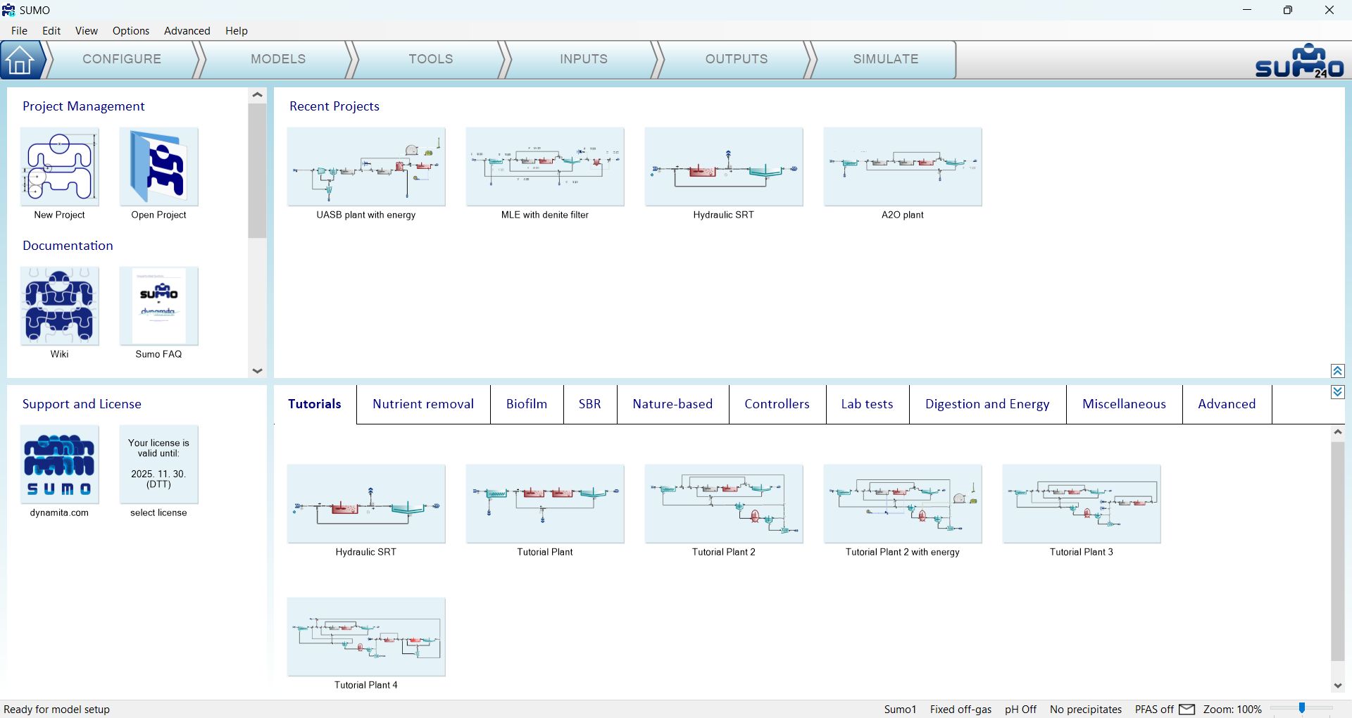
The central elements of the SUMO Welcome Screen are four screen panels, whose functions and roles are the following:
| Top left panel |
Project management and documentation Starting or opening a new project in a new window (New Project), opening a saved project from your own files (Open Project) and reaching various documents for how-to-use instructions. |
| Top right panel |
Recent projects Your recently opened projects can be quickly reached from the welcome screen. |
| Bottom left panel |
Support and license information SUMO support (link to our website) and the currently used license information can be reached from here. |
| Bottom right panel |
Built-in example project repository All the built-in example configurations can be opened directly from this pane (they are also available from the Help menu). |
These functions can be reached later at any point, by clicking either the Home icon (the first item of the Task Bar) or the SUMO24 logo (located at the right end of the Task Bar), which will bring you back to the Welcome Screen.
The screen panels can be resized anytime during the workflow to fit the actual needs of the job. In order to do that, just move the mouse to the padding between the panels and drag them to the desired position. The top right panel will always contain the plant configuration, while the content of the other panels depends on the actual task (Configure, Modes, Tools, Inputs, Outputs, and Simulate). Please note that the runtime versions of Sumo are not meant for constructing new models and thus, the Configure, Models and Tools tabs are not available.
The Status Bar in the bottom of the screen provides model/simulation related information. In case of a system notification or model/simulation error, an exclamation mark will appear next to the mailbox icon (Figure 2.1.2). Red exclamation marks denote errors, while blue and yellow ones inform about warnings and notifications that need attention. Clicking on the mailbox icon will provide the description of the problem and hints about dealing with it.

The following chapters will help you to understand the functions of each main tab of the Task Bar, and teach how to use them for building a project and performing various simulations.
¶ Configure
To start your project, click on the New Project icon or the Configure tab. This task serves the building of the plant layout.
The roles of screen panels in Configure mode are the following:
| Top right panel | Plant configuration drawing board |
| Top left panel | Process unit categories and process units |
| Bottom right panel | General comment panel – your notes, which will be saved with the project |
| Bottom left panel | Specific process unit options and information |
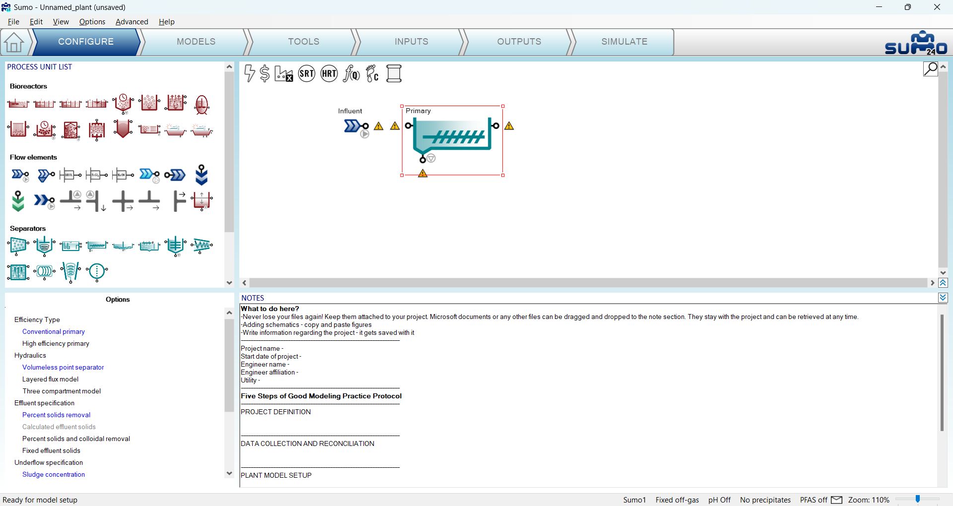
While the Configure tab is selected, we will build a simple AO configuration (also available for reference from the built-in examples as Tutorial plant) using the Flow elements, Bioreactors and Separators categories from the top left element list. Select the desired process unit by opening the category and dragging the process unit to the drawing board. To drop the selected unit, just release the mouse button (Figure 2.2.1).
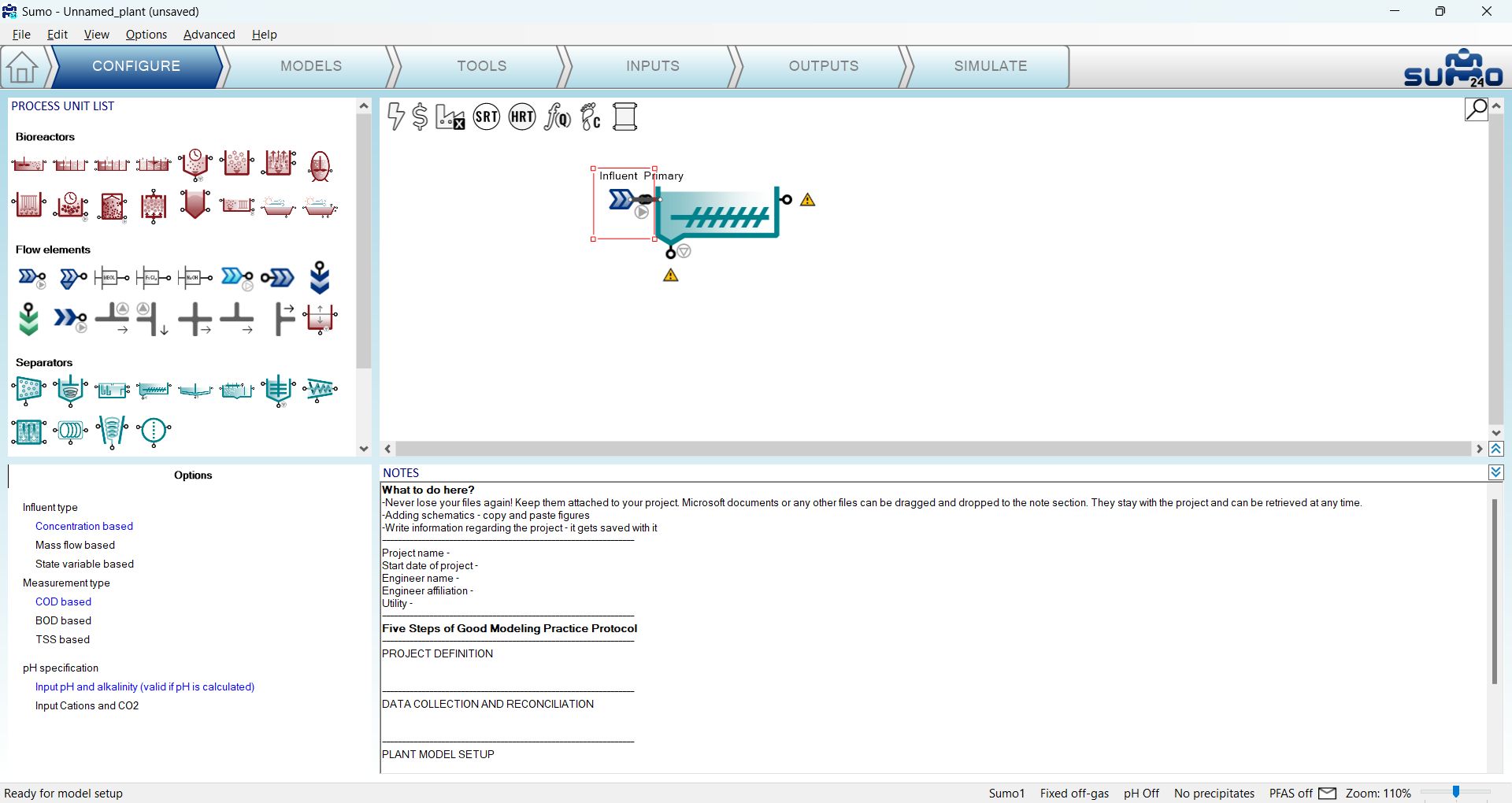
Pipes can be created using two methods. Sumo supports a handy way of establishing connections between process units, which can be triggered by positioning a process unit’s output port on top of another process unit’s input port (or vice versa) by moving one of the process units. Once the ports are positioned on top of each other, a pipe connection is automatically created, as it is demonstrated by Figure 2.2.2 with an Influent and a Primary clarifier. This method is especially useful when Sumo is commanded by fingers on a touch screen. Unconnected ports are indicated by yellow exclamation marks in the Configure and Models tabs.
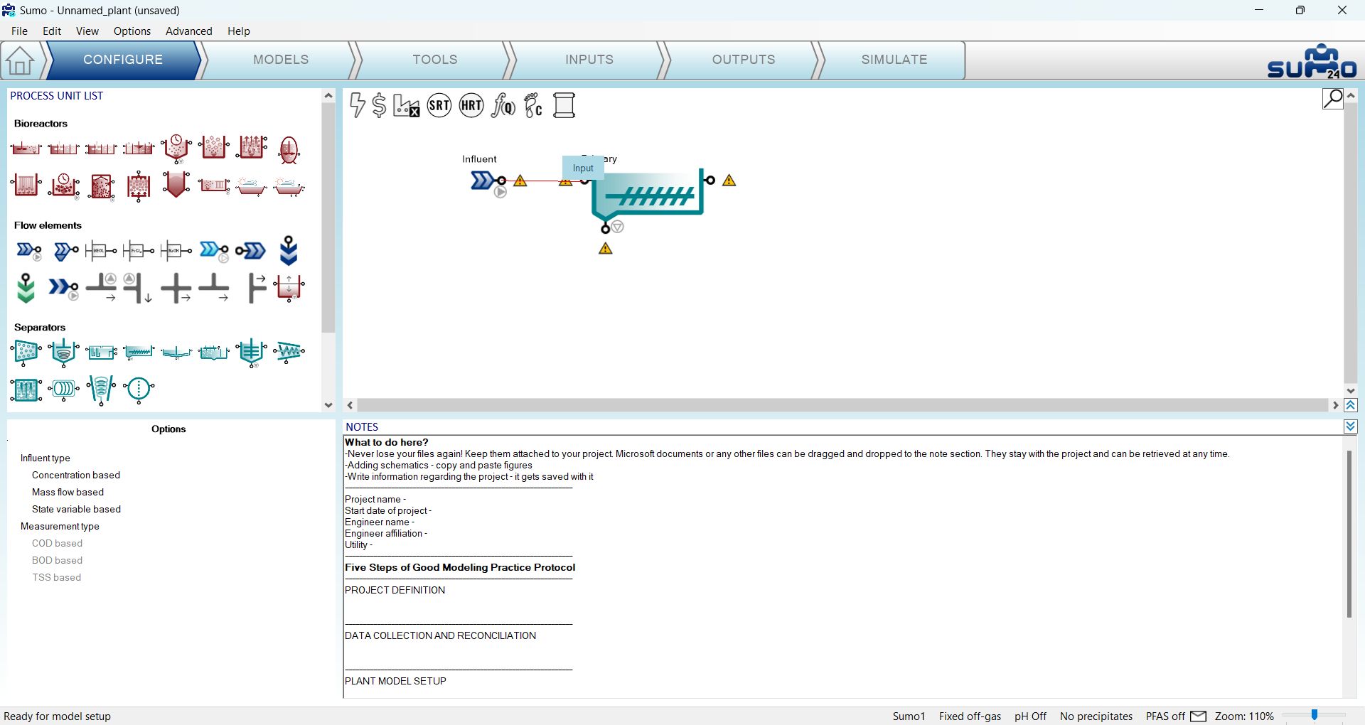
The conventional way also works: position the mouse on an output port of a process unit, press the left mouse button, then move the mouse – and this way drag the pipe, denoted by a red line – to an input port of another process unit (as illustrated in Figure 2.2.3) and finally release the mouse button to make the connection. Existing pipes can be removed by right clicking on them and selecting Disconnect pipe from the pop-up menu.
Build the plant configuration and connect the pipes as shown by Figure 2.2.4. Tooltips provide hints about the purpose of a unit’s connection point. This feature comes especially handy for the flow divider and flow combiner (make sure not to mix up these connections – their name is shown on a pop-up tooltip and flow direction is indicated by small arrows). Rotate the flow divider below the clarifier by swiveling the red selection rectangle (or with a right click pop-up menu option) and straighten the lines by grabbing process units or pipe corners. These maneuvers do not change the results of the simulation but will make working with the model a lot clearer.
Upon selecting a process unit on the drawing board, options appear in the bottom left panel, where the most suitable process unit can be chosen, fitted to the model. In this Tutorial we will use:
Table 2.2.1 – Components of the Tutorial Plant
| Influent | |
| Influent type | Concentration based |
| Measurement type | COD based |
| pH specification | Input pH and alkalinity (valid if pH is calculated) |
| Primary | |
| Efficiency type | Conventional primary |
| Hydraulics | Volumeless point separator |
| Effluent specification | Percent solids removal |
| Underflow specification | Sludge concentration |
| Reactions | Non-reactive |
| CSTR (both) | |
| Dissolved oxygen | Input |
| Aeration | Diffused |
| Reactor type | Mainstream |
| α factor specification | Predicted α |
| Diffuser system specification | Membrane discs |
| Reactions | Reactive |
| Clarifier | |
| Efficiency type | Conventional clarifier |
| Hydraulics | Volumeless point separator |
| Type of clarifier | Final clarifier |
| Effluent specification | Fixed effluent solids |
| Underflow specification | Sludge flow |
| Reactions | Non-Reactive |
| Side flow divider | |
| Flow divider options | Side flow divider with side pump (with cycling turned off) |
Note: The flow divider’s connection where the small pump symbol points to needs to be connected to the waste sludge and the other output (where the arrow points to) will be the recycled activated sludge.
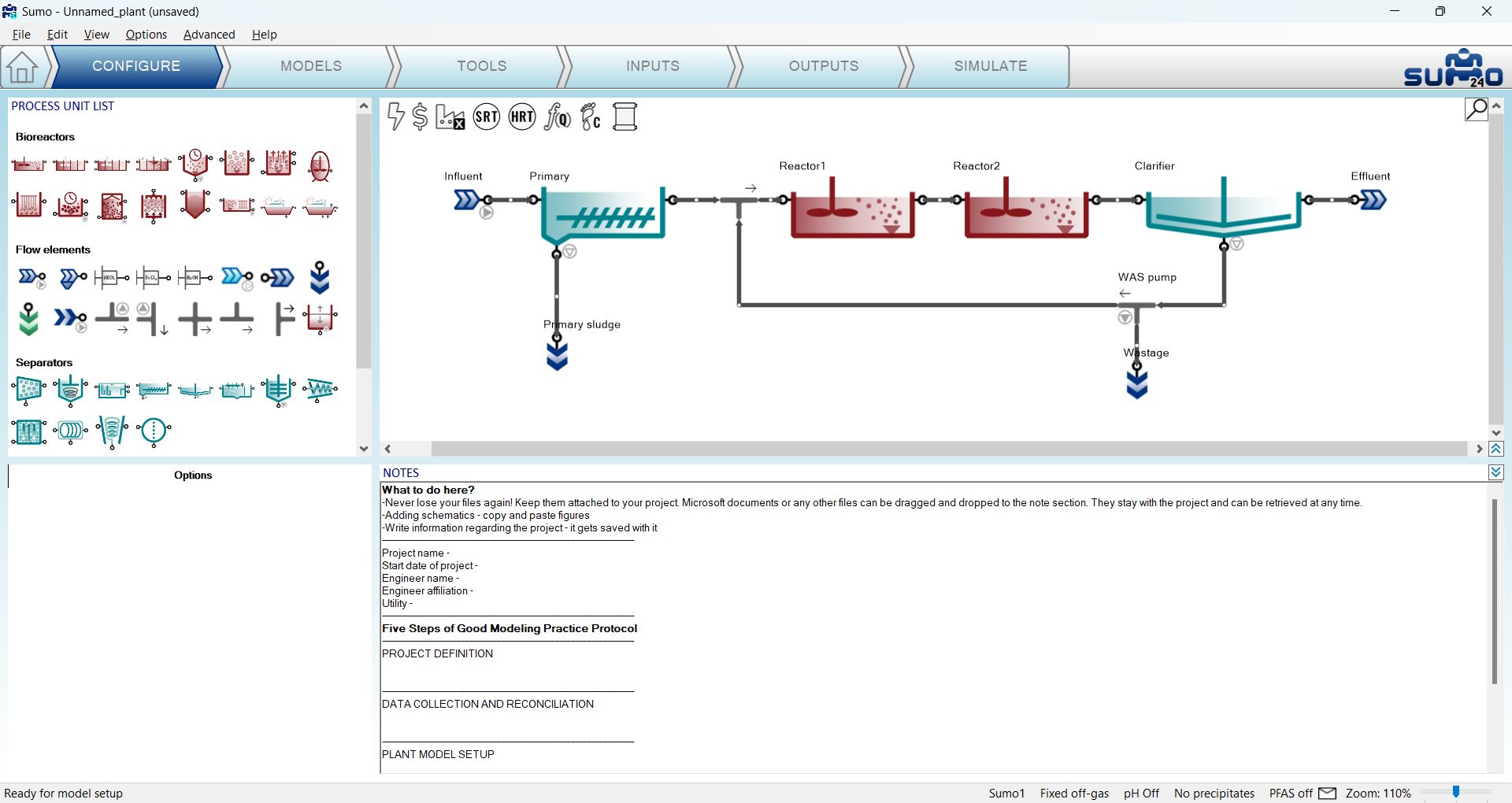
The drawing board can be easily zoomed in and out by holding down the CTRL key while scrolling with the mouse wheel, or alternatively by adjusting the zoom slider in the right end of the Status Bar. To move the configuration around the pane, hold down the CTRL key and the middle mouse button simultaneously while moving the mouse. To fit the actual configuration in the center of the viewport with the optimal zoom level, press CTRL+Home.
Rename the process units using the right-click pop-up menu, the F2 function key or double-click on the upper part of the unit. The pipes can be renamed as well, but this is usually not important – the pipe names are hidden by default (this can be changed in the View menu on the top). The visibility of process unit names can be controlled on a one-by-one basis. In order to obtain a clear example layout, hide the name of the ‘Side flow combiner’ process unit (this is the default setting).
Note: the above settings can only be modified in Configure mode, but you can return and perform them at any point during your work. Changing the process unit names will not result in recompilation of the project model.
Note: other process units (e.g. Sewer network and Mobile carrier) may be available as add-ons. Please write to support@dynamita.com for information.
¶ Models
In this optional task, the mathematical model describing the biological, chemical and physical processes can be selected. If no settings are changed, the default settings will be used – the model will be functional.
The role of screen panels in Models mode are the following:
| Top right panel | Plant configuration |
| Top left panel | Available model options or models in advanced mode |
| Bottom right panel | Model parameters |
| Bottom left panel |
Model parameter categories Note: in the case of Sumo models, only selected key parameters are shown by default; click on the Show all button to see the entire parameter set. |
In this task, we can choose between using the various built-in models for our plant, as well as additional options like turning on or off gas phase, precipitation and different complexity levels of pH calculations.
The current package comes with the Sumo whole plant models listed in Table 2.3.1.
Table 2.3.1 – Description of Sumo whole plant models
| General full plant models | |
| Mini_Sumo |
Simplified One step whole-plant model Use “Mini_Sumo” for OUR and sludge production prediction. |
| Sumo1 |
One step whole-plant model Use "Sumo1" for activated sludge modeling, iron addition for P removal and with plants that have digesters but no iron addition. |
| Sumo2 |
Two step whole-plant model Use "Sumo2" for activated sludge modeling and sidestreams, iron addition for P removal and with plants that have digesters but no iron addition. |
| Focus models | |
| Sumo2S |
Two step whole-plant model Use "Sumo2S" for whole plant modeling, (activated sludge, digesters, sidestreams), particularly if iron is dosed and is carried to the digester with the sludge. This is the only model which includes the full interaction of the sulfur and iron cycle. |
| Sumo2C |
Two steps whole-plant model - High rate Use "Sumo2C" for high rate activated sludge modeling and sidestreams, iron addition for P removal and with plants that have digesters but no iron addition. |
| Sumo4N |
Four step whole-plant model Use "Sumo4N" for whole plant modeling, (activated sludge, digesters, sidestreams) when particularly interested in GHG emissions for carbon footprint estimations. |
The general full plant models are available directly from the Model selection list (top left panel), while the focus models (and other custom models) are accessible either by choosing the Museum, Focus and custom models item, or by clicking the Advanced button (located in the bottom of the top left panel) – both will open up the complete Model library in the top left panel. When the Model library is shown, right-clicking on the model name will enable opening the source code in SumoSlang (Excel) format (Figure 2.3.1). To return to Model Options from here, just hit the Back button in the bottom part of the screen panel.
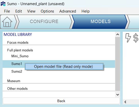
Table 2.3.2 lists the main processes included in the Sumo whole plant model family.
Table 2.3.2 – Main processes included in Sumo whole plant models
|
General full plant models |
Focus models |
|||||
|---|---|---|---|---|---|---|
|
Mini_Sumo |
Sumo1 |
Sumo2 |
Sumo2S |
Sumo2C |
Sumo4N |
|
| COD removal |
X |
X |
X |
X |
Two populations: OHO and AHO |
X |
| EPS production |
|
|
|
|
X |
|
| Denitrification |
1-step |
1-step |
2-step |
2-step |
2-step |
4-step |
| Hydrolysis |
X |
X |
X |
X |
X |
X |
| Fermentation |
X |
X |
X |
X |
X |
X |
| Anoxic methylotrophs |
|
X |
X |
X |
X |
X |
| Nitrification |
1-step |
1-step |
2-step |
2-step |
2-step |
4-step |
| EBPR (PAO-GAO model) |
|
X |
X |
X |
X |
X |
| Three-population anaerobic digestion |
X |
X |
X |
X |
X |
X |
| Temperature sensitivity |
X |
X |
X |
X |
X |
X |
| Precipitation |
|
X |
X |
X |
X |
X |
| Chemical P removal |
based on ASM2d approach |
Kinetic approach |
Kinetic approach |
Kinetic approach |
Kinetic approach |
Kinetic approach |
| Sulfur cycle |
|
|
|
X |
|
|
| GHG emissions |
|
|
|
|
|
X |
Important comment on Mini_Sumo: unlike other Sumo whole plant models, Mini_Sumo does not include colloidal components. The user should pay careful attention on the influent fractionation and – if required – primary clarifier calibration, so that the primary effluent composition in terms of BOD and TSS is in agreement with the expectations.
Note: other models may be available as add-ons. Please write to support@dynamita.com for information.
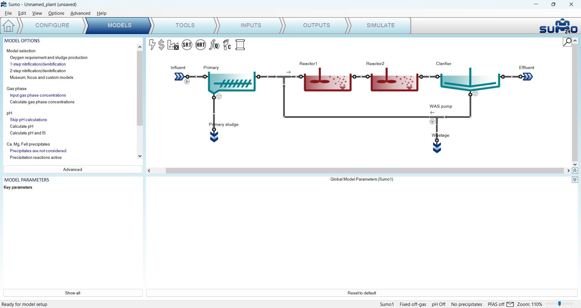
In our example we will use the default model setup with one step nitrification-denitrification model (Sumo1) with specified input gas concentrations (gas transfer is approximated, off-gas concentrations are fixed) and without pH calculation or chemical precipitation, as shown in Figure 2.3.2.
¶ Global model parameters
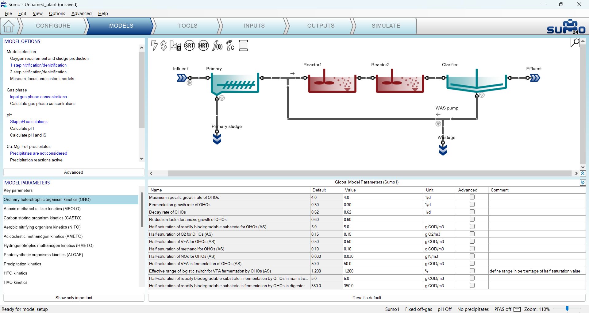
On the Models tab, if none of the process units are selected, clicking on the parameter categories listed in the bottom left panel (remember to click the Show all button in order to access all parameter tables in Sumo models), global kinetic and stoichiometric model parameters can be reviewed/modified. Each table will open up in the bottom right panel. This way the model parameters can be set globally, for the whole plant (Figure 2.3.3). These parameters will not be changed in this tutorial.
¶ Local model parameters
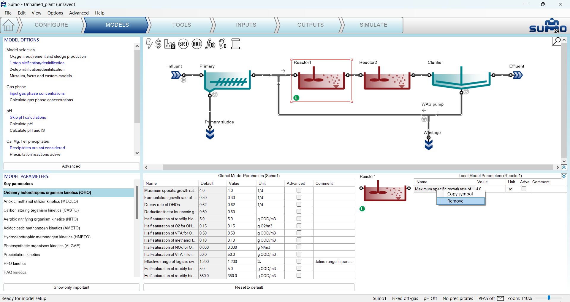
Any model parameter can as well be set as a process unit specific “local parameter”, by selecting the unit and dragging the desired parameter to the right side of the bottom right panel, as shown on Figure 2.3.4. In this case, the process unit will get a green “L” mark to remind the user for the local changes. Local model parameters will NOT be used in the current example, the aim of the above description was to explain this advanced functionality. You can remove local parameter selection by right clicking on the name of the parameter and selecting Remove.
¶ Tools
Proceeding to the Tools tab, complex plantwide calculations can be defined (Figure 2.4.1).
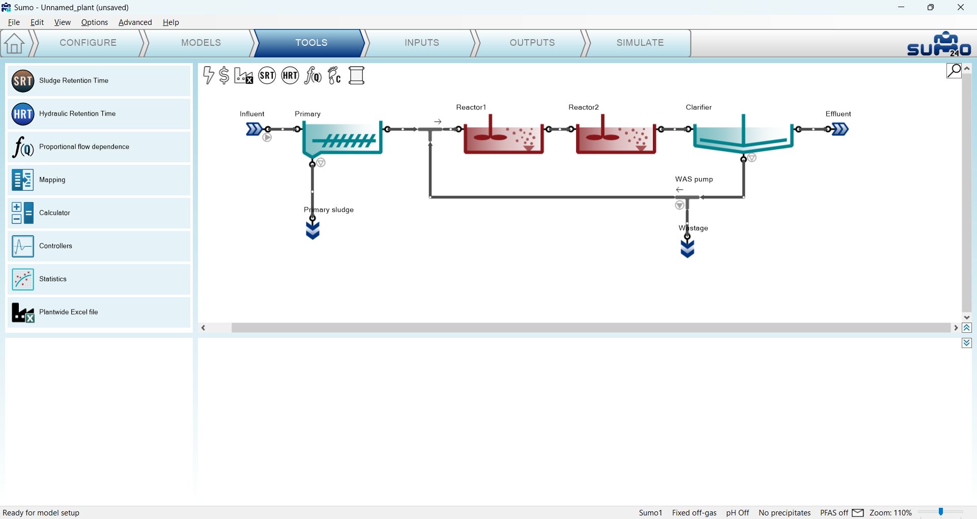
“Plantwide” means that the calculations are based on variables contained in several process units around the plant. The following calculations can be added to the simulation (listed in the top left panel):
- Sludge Retention Time
Plant specific SRTs (total, aerobic, etc.) can be calculated.
- Hydraulic Retention Time
Plant specific HRTs can be calculated
- Proportional flow dependence
Plant specific flow dependence (e.g. RAS flow as percentage of influent flow) can be defined.
- Mapping
Parameters can be mapped from one process unit to another one.
- Calculator
Variables (e.g. volumes, masses) can be summed up in the plant. Simple and advanced variable ratios can be defined for the plant (e.g. N removal efficiency = effluent TN/influent TKN).
- Controllers
Controllers allow the user to configure automatic control (such as time based on/off, PID etc.) of process unit parameters.
- Statistics
A few statistical options (Moving average, Noise generator, Totalizer ) are available here.
- Plantwide Excel file
The plantwide code is not confined to one process unit (PU) but can use variables from all over the plant model. The plantwide code file can be opened from the GUI directly. Further information and an example can be found in the Technical Reference document.
¶ Sludge Retention Time
The SRT calculation is set up the following way: drag reactors that contain sludge mass to the numerator and drag wastage – and if desired, effluent connections (ports) – in the denominator, as illustrated by Figure 2.4.2.
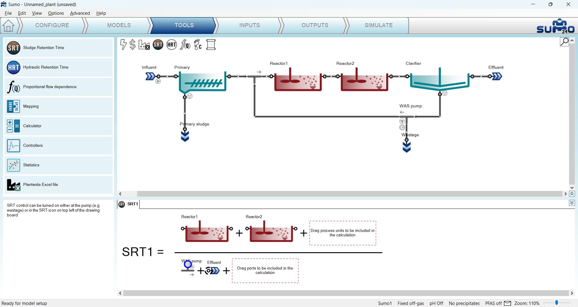
Several SRT calculations can be set up, e.g. total and aerobic, or North and South side SRT, etc. In this tutorial the total plant SRT will be calculated (as shown on Figure 2.4.2).
Note: When the project has an SRT calculation, the SRT icon on top of the drawing board gets a brown color.
Target SRT can be defined as well, by assigning a proper controlled port. These ports, such as the WAS pump in our example, are indicated by a “C” sign within a blue circle. A certain pump can only be used to control one SRT. Pumps can be selected and deselected for SRT control by right clicking their icon in the equation and choosing the desired option. When a pump is selected for control, Remove Controlled will deselect it (the “C” sign will disappear from the blue circle), while non-controlling pumps can be set to be controlling ones by choosing Mark as Controlled (Figure 2.4.3).
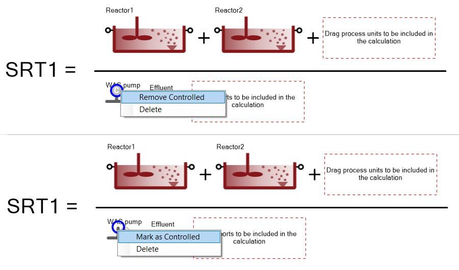
Note that even though the wastage pump is selected for SRT control, it has not been designated yet for this role at the current stage (this is indicated in the plant layout by a grey “C” sign next to the pumped outflow pipe of the WAS pump). The activation of the SRT control can take place in a subsequent step (see the Plantwide inputs chapter).
¶ Hydraulic residence time
The HRT tool is meant to calculate the plantwide hydraulic retention time with specific tank volume (of single tank or multiple tanks) and plant influent flow rate. Several HRT calculations can be set up, e.g. total, anoxic, aerobic, or HRT of one of the parallel trains, etc.
A ratio is involved to define the respective flow rate for each train when there are parallel trainings in the treatment process splitting the influent flow (if there's only one train, the ratio should be 100%), and it can be steady or dynamic. For steady ratio, the value can be set under INPUTS. For dynamic ratio calculation, you can use the "Ratio of variables" in the Calculator category under TOOLS, and map the calculated ratio to this equation. We will set up an HRT calculation for this plant at a later stage of this tutorial.
¶ Sum of variables
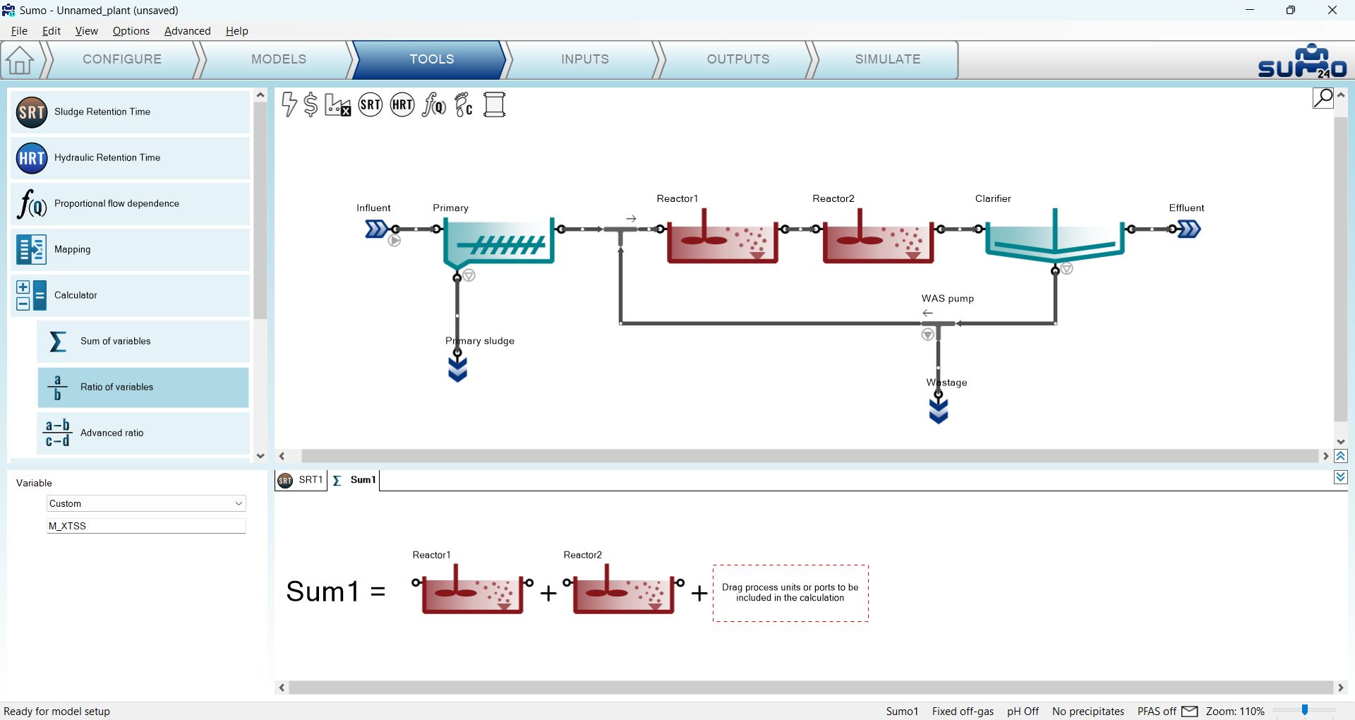
For calculating the Sum of variables, a set of predefined items are available (organized into groups) from dropdown menus in the bottom left panel. If the desired variable cannot be found here, custom variable input can be used well (choosing the last item in the first dropdown menu). In the latter case, make sure that the correct symbol is used, otherwise the built-in GUI check will disallow the calculation. Symbols of variables can be figured out using various methods (hints will be given in a subsequent chapter; details of the naming convention are described in the Technical Reference).
In this example, we will calculate the sum of Suspended solids mass in the reactors by entering “M_XTSS” as custom variable and dragging Reactor 1 and Reactor 2 into the equation from the layout (Figure 2.4.4).
¶ Ratio of variables
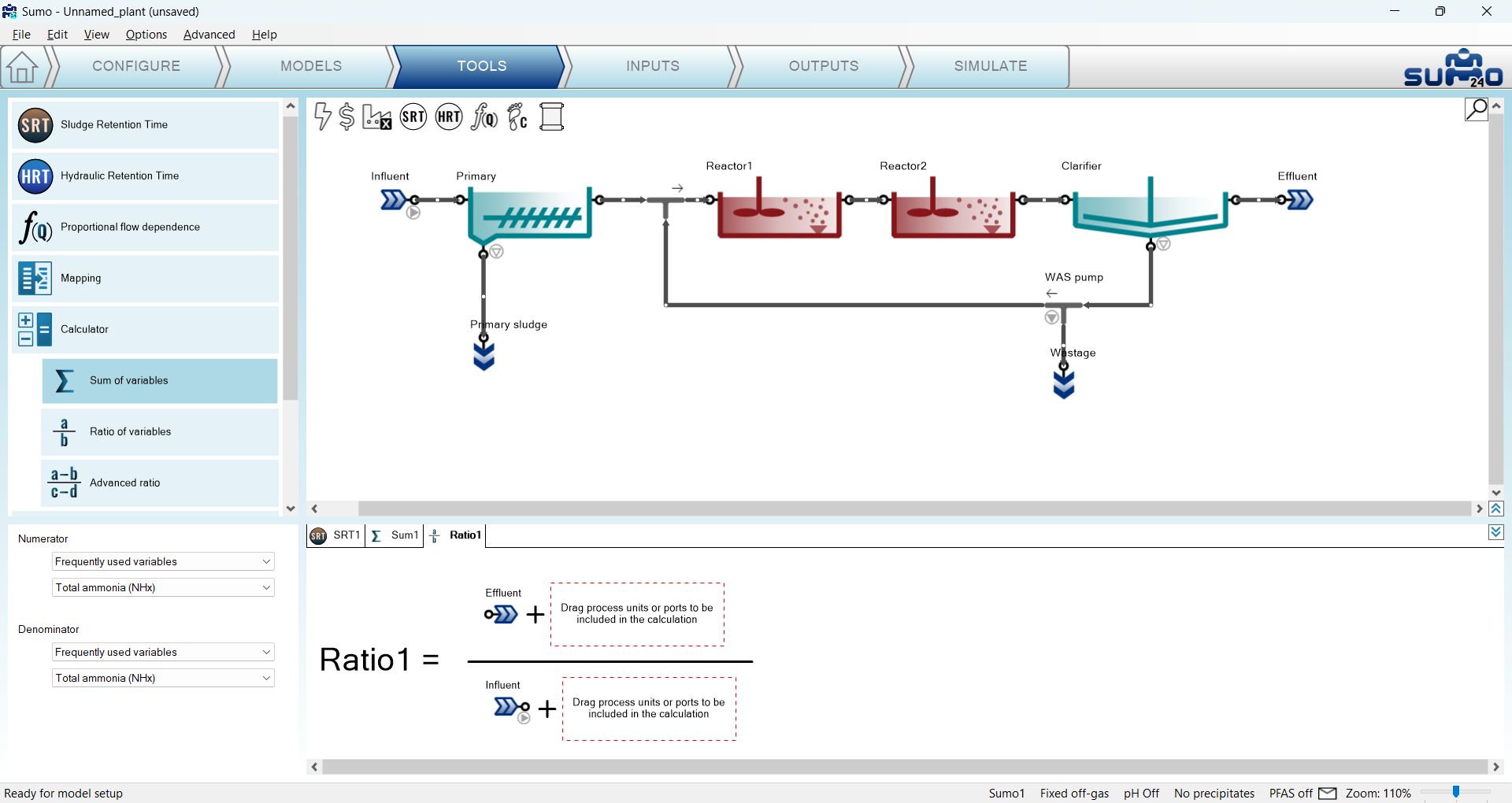
Adding Ratio of variables can be done in a similar way as the Sum of variables. First select the variables to be used in the numerator and the denominator from the dropdown lists of the bottom left panel, then drag the desired process units to the ratio. In this example, we will calculate the removal ratio of Ammonia, as shown on Figure 2.4.5.
¶ Proportional flow dependence
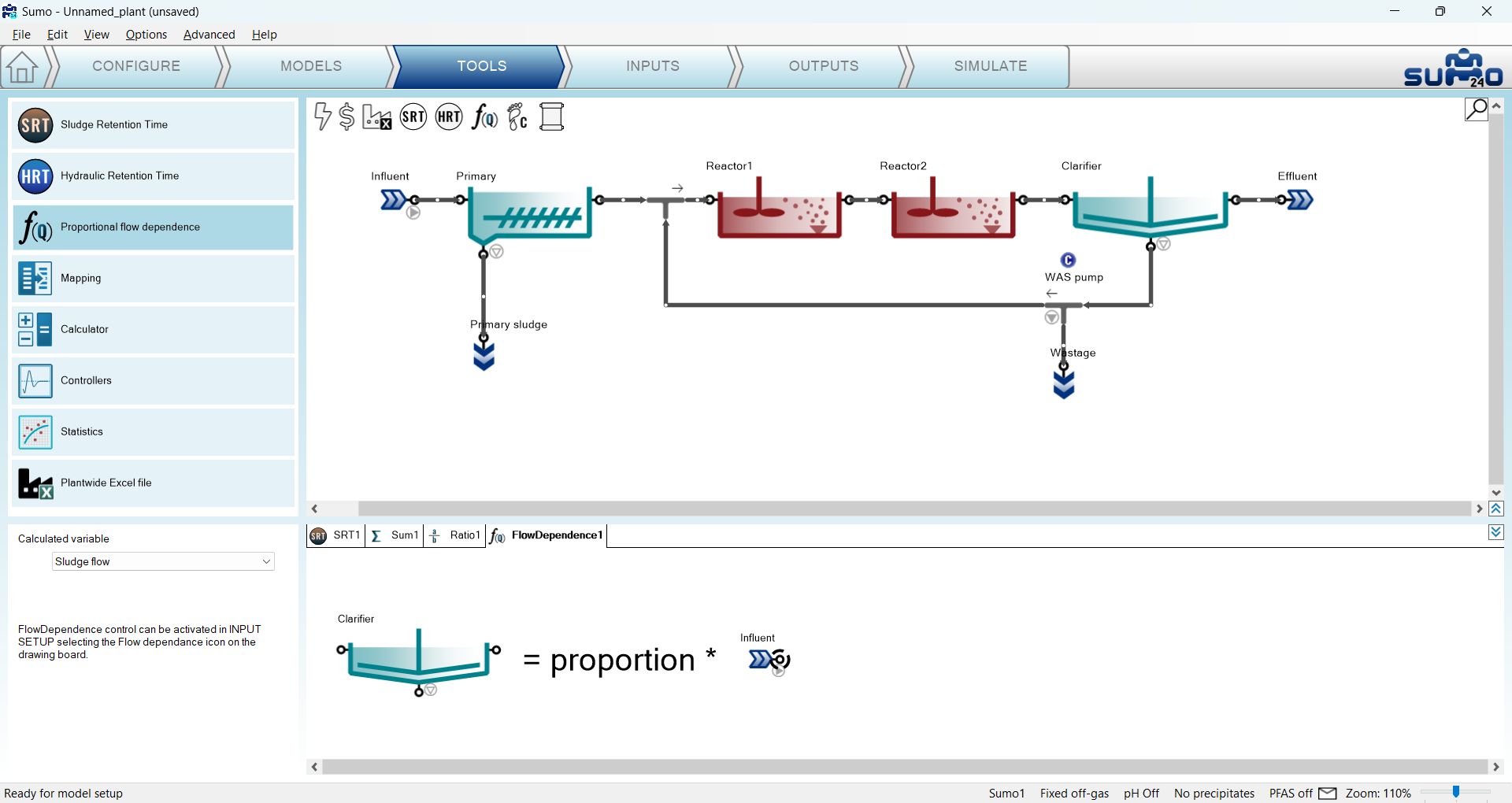
Adding Proportional flow dependence can be done by dragging the desired process units to the respective slots of the dependence equation. In this example, we are going to set the clarifier sludge recycle flow to be proportional to the influent flow rate, as shown on Figure 2.4.6. You will see a blue “C” sign showing up beside the clarifier on the drawing board, indicating that its sludge flow became a dependent parameter (controlled by the influent flow). The exact value of the proportional dependency will be set in a subsequent step (see the Plantwide inputs chapter). The controlling flow (e.g. influent) must not be within the loop (i.e. 50% of clarifier input flow to set the RAS flow cannot work as there is no solution to that loop).
Note: When the project has a proportional flow dependency, the “Q” in the f(Q) icon on top of the drawing board gets a blue background.
¶ Controllers
Controllers help to keep certain operational parameters of the selected process unit at a required setpoint or within a band. The following controllers are integrated into SUMO24 (Figure 2.4.7).
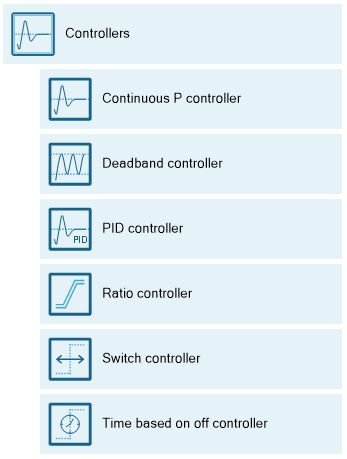
In this example, we will use a Deadband controller to control the sludge wastage pump automatically, in order to maintain the MLSS between certain limits. Details about the further controller options can be found in the Controllers chapter.
¶ Deadband controller
Adding a Deadband controller can be done in a similar way as the Sum of variables. First drag and drop the manipulated unit to the left side of the equation in the bottom right screen panel, and then the controlling unit to the right side of the equation. In the bottom left screen panel, you can now select the control variable (CV) and the manipulated variable (MV, a parameter) of the selected units. In this example, we will manipulate the Wastage pump to achieve the desired MLSS range, see Figure 2.4.8. Note that the “C” sign by the wastage pump will change to blue color, indicating that we have just set up and designated a controller for it that took over the role of the previously defined (but not activated, hence the former grey color) SRT control.
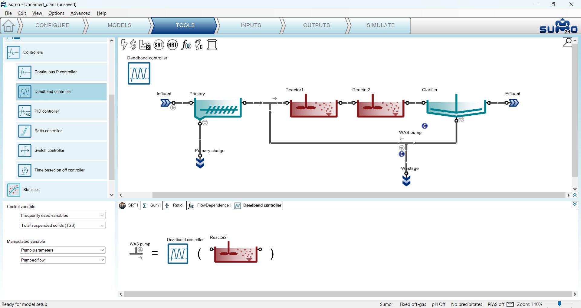
The controller image that appears in the plant layout can be repositioned on the drawing board by holding the CTRL key while the icon is being dragged and moved, so the layout can be better understood. Move the controller icon above Reactor 2, then select it and hit F2 (or alternatively, right click on the tab header in the bottom right panel) to rename it to “MLSS control by WAS”. This will rename the respective tab (or the controller icon) as well.
¶ Statistics
The Statistics section contains calculations for easier understanding or presentation of the results, such as average or totalized calculations. The following statistical calculations are integrated into SUMO24 (Figure 2.4.9).
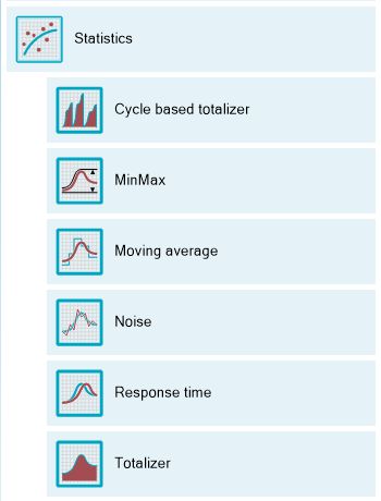
As an example, we will set up the average effluent concentration of the plant.
¶ Moving average calculation
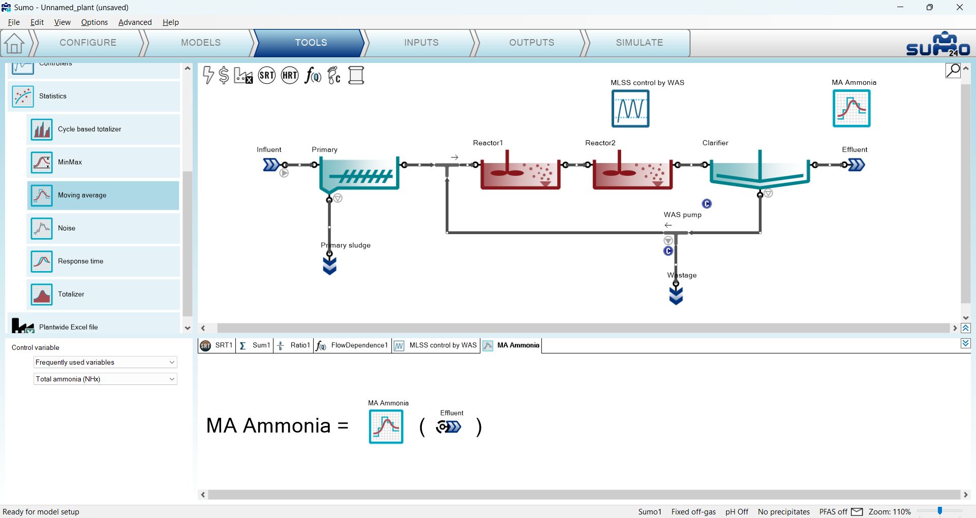
Moving average can be added in a similar way as Sum of variables. First drag and drop the process unit to which the calculation should apply, to the right side of the equation on the bottom right panel. In the bottom left panel you can now select the desired variable whose average should be calculated. In this example we will calculate the average effluent ammonia concentration, see Figure 2.4.10.
The statistical unit image can be repositioned on the drawing board and renamed similarly to controllers. Move the icon above the Effluent and rename it to “MA Ammonia”.
¶ Inputs
Choosing the Inputs task, the blue workflow tab above the drawing board automatically splits into Constants and Dynamics. According to this, different types of settings become available: we can set either constant inputs (e.g. fixed influent composition, reactor DO setpoints etc.) or dynamically changing inputs (e.g. variable influent flow, composition, shifting reactor DO setpoints etc.). At this point, Sumo will be compiling your model in the background (you can track the progress in the Status Bar). However, in most cases, you can already start providing information to Sumo. When your layout requires using arrays (e.g. layered clarifiers, biofilm), please wait until the model is fully compiled and loaded (status bar message: “Ready for Simulation”). For the initial plant setup, we will only need the Constants, as shown on Figure 2.5.1. Select each object one by one and enter the required values as shown below.
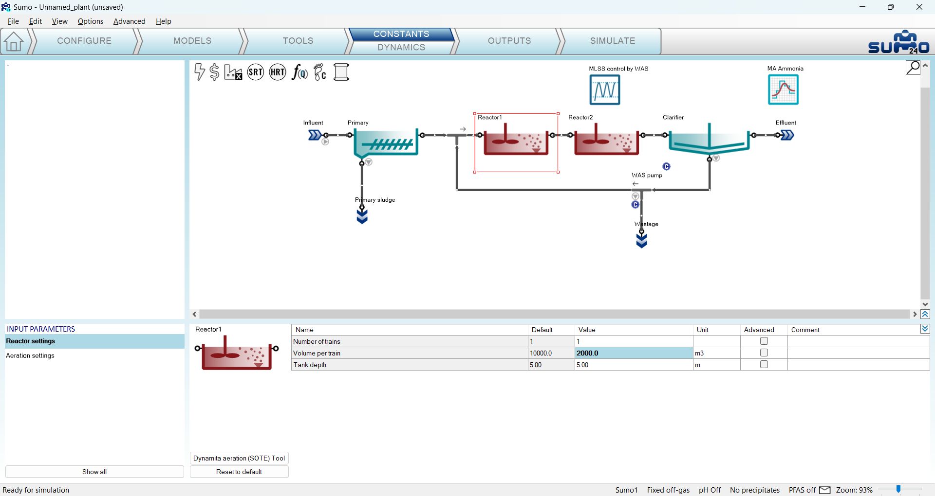
In this simple configuration, we only need to set a few values to build a realistic plant model, first for typical dry weather operation. Use the values from Table 2.5.1 for this example (leave everything else at default):
Table 2.5.1 – Input setup for AS plant
| Process Unit | Parameter group | Parameter | Value | Unit |
| Reactor 1 | Reactor settings | Volume per train | 2000 | m3 |
| Reactor 2 | Reactor settings | Volume per train | 8000 | m3 |
| Influent | Influent specifications | Flow rate | 20000 | m3/d |
| Influent | Influent specifications | Total COD | 500 | g COD/m3 |
| Influent | Influent specifications | Temperature | 22 | °C |
Enter these values by selecting the respective process unit on the drawing board and the parameter group in the Input parameters menu (bottom left panel) – the values can be edited in the bottom right panel (Figure 2.5.2). Each value that is different from the default will be highlighted with bold letter type. There is also a similar indication in the Input parameters menu for parameter groups that contain non-default values.
Whenever the entered value is out of the allowed range specified in the model, Sumo will notify you with a prompt window and set the value to the nearest feasible bound, indicating the automatic choice by applying red color to the text. This value can be overridden manually with a valid number.
If needed, all changes applied to the values of the actual parameter group can be reverted to defaults by clicking the Reset to default button located in the bottom right screen panel (Figure 2.5.2). Also, there is a unit conversion module for US units (MGD, scfm, etc.) in the Options menu item if needed.

For setting the plant specific influent composition, the use of the Influent tool Excel file is recommended. The Influent tool can be reached directly from the input setup of the Influent, by clicking the button located in the bottom right screen panel (Figure 2.5.3). The details of the Influent tool are described in the Influent tool section. At this point, we will not alter the influent composition, so we will skip using the Influent tool.
Parameters for scenario runs and scenario analysis (as well as for optimization) can be selected by using the checkboxes in the Advanced column. In this example, we will select the influent Flow rate, Total COD and the Temperature parameters (Figure 2.5.3). The use of scenarios will be described in the Scenario runs chapter.

The controller parameters can be setup at this stage as well. In this Deadband controller example, we will set:
- Controller direction: inverse (-1), since increasing wastage (MV) will decrease MLSS (CV), i.e. the CV responds inversely to MV change;
- 2600 mg/L as low value and 2800 mg/L as high value for the Controlled variable (MLSS in Reactor 2) range;
- 150 m3/d as low value and 600 m3/d as high value for the Manipulated variable range (the latter represents the physical pump capacity for the Wastage pumped flow);
- Initial value of manipulated variable to single pump capacity as 150 m3/d.
See these settings on Figure 2.5.4.
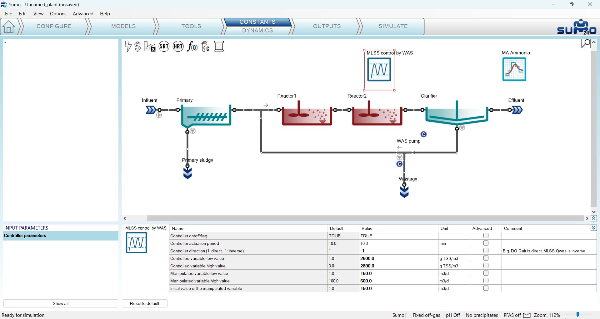
The input setup of this wastewater treatment plant model is now ready.
¶ Influent tool
The Influent tool is a multiple sheet Excel file to help to set up the proper influent composition. The role of each sheet is explained in Table 2.5.2 below.
Table 2.5.2 – Description of the Influent tool
| Influent tool sheets | |
|---|---|
| Help | Short description of the file content |
| Data | Input of the available measurement data of the simulated plant or facility. This sheet provides help to estimate the missing data based on available information for municipal or industrial wastewater composition. |
| Check fractions | On the left side of the sheet, the estimation of key organic fractions is available, such as COD and N fractions, particulate COD/VSS ratios by component, yield on ultimate BOD and BOD fraction for soluble, colloid and particulate. On the right hand side, the calculated COD, BOD5 and TSS/VSS values can be checked if they match the measured values. |
| Sumo forms | This sheet gathers all the information that can be used to simply copy into the Sumo Models or Inputs tab of the Influent process unit. |
| Fractionation tree | This sheet shows the fractionation graphs of total COD, suspended solids, N and P based on your input data, helping to visualize the organization of the individual fractions used in the model. |
| Balances | On this sheet, the organic compounds can be checked (how the fractions add up to the total). The sheet will also provide warning when negative component concentrations result from the estimated fractions (such as not enough N for organic TKN if most of TKN is ammonia, and there are solids in the influent) |
| Diurnal flow | This sheet provides example and usual flow pattern for small, medium and large plants. Based on the influent value, the diurnal flow dynamic input tables are prepared for copy and paste into Sumo. |
| Birthday cake | On this sheet, you will find a ready-made table for a “birthday cake” type of load analysis, prepared from your input and diurnal flow data. |
| Calculations | This sheet contains the details of BOD calculation and the error tolerances used on Check fractions sheet. |
For a detailed description of the Influent tool please refer to the Tools in Sumo chapter of the Technical references, and guidelines for influent fractionation are available in Influent characterisation chapter.
¶ Dynamic Inputs
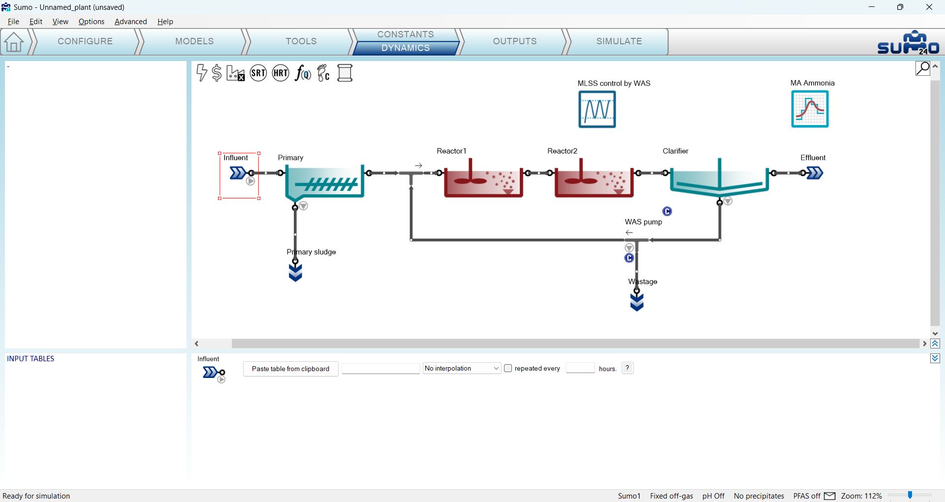
This optional task can be used to enter dynamically changing input information, e.g. diurnal flows, DO schedules and more. To activate the dynamic input setup, click on the lower part of the Inputs tab on the Task Bar, labeled as Dynamics (Figure 2.5.5).
The role of screen panels in Dynamic Inputs mode are the following:
| Top right panel | Plant configuration |
| Top left panel | Unused in this mode |
| Bottom right panel | Data entry functionality |
| Bottom left panel | List of entered dynamic data tables |
If we wish, we can copy and paste entire data tables from an Excel file into Sumo. This will be discussed later in the Subjecting the plant to dynamics section.
¶ Plantwide inputs
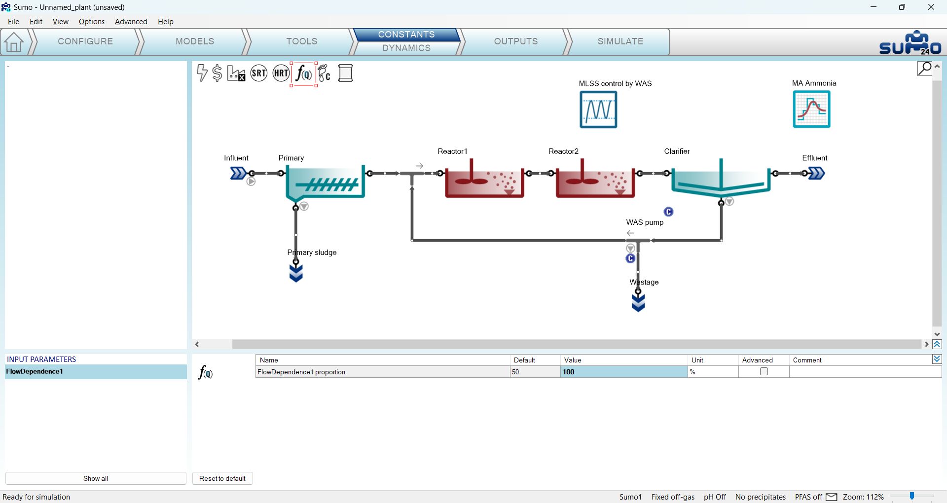
Target SRT and proportional flow dependence input settings can be accessed by clicking on the respective icons listed on the top left part of the layout panel. In this simulation, we will not use the Target SRT controller, but will set up the proportional sludge flow of the clarifier to 100%, as shown on Figure 2.5.6. This will align the sludge flow rate with the influent flow as 1 to 1.
The plantwide parameters set in the Plantwide Excel file will appear in the Inputs tab when the plantwide (factory) icon is selected in the top section of the layout. These can also be changed dynamically, similarly to any other model parameter (for more detailed information on this feature, please consult the Technical Reference). In this simulation, we will not use plantwide parameters.
¶ Outputs
This task can be used to specify which variables and in what format should be displayed and/or saved during the simulation phase (Figure 2.6.1).
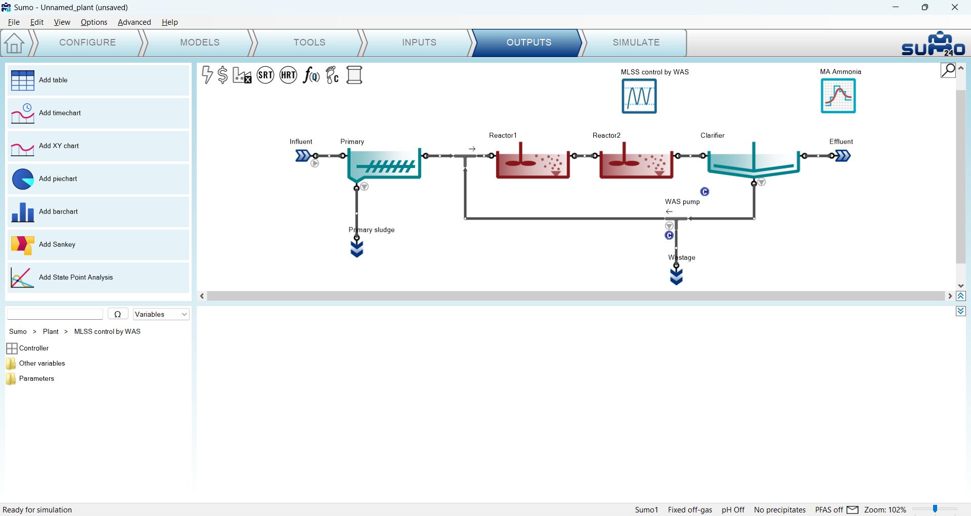
The role of screen panels in Outputs mode are the following:
| Top right panel | Plant configuration |
| Top left panel | Buttons for different diagram types (Table, Timechart etc.) |
| Bottom right panel | Added outputs in a series of tabs |
| Bottom left panel |
Output variable list for the selected unit and the connected pipes Available once the model is fully compiled. The user can browse the variables based on their name or symbol. There are also preselected categories (frequently used, operational variables etc.) available to help the work. |
¶ Adding a table
Click the Add table button in the top left panel: this will add a table to the bottom right panel. The table can be renamed (right click on the tab and choose Rename from the pop-out menu or simply just double-click on the tab) and several tables can be added. Name this table “Results”. Add process units to the table by dragging them to the table (by selecting multiple units in the drawing board, they can be added in one go as well). Add variables to the table by selecting and dragging them from the bottom left panel (Figure 2.6.2). Entire display tables can be added at once by dragging the prepared table e.g. Frequently used variables (Note: if the table has not been renamed by the user, it is automatically renamed when a whole display table is added). The exact list of preselected variables varies according to the process units (in this example, the Influent was selected when adding Frequently used variables to the table). Initial values will appear in the cells.
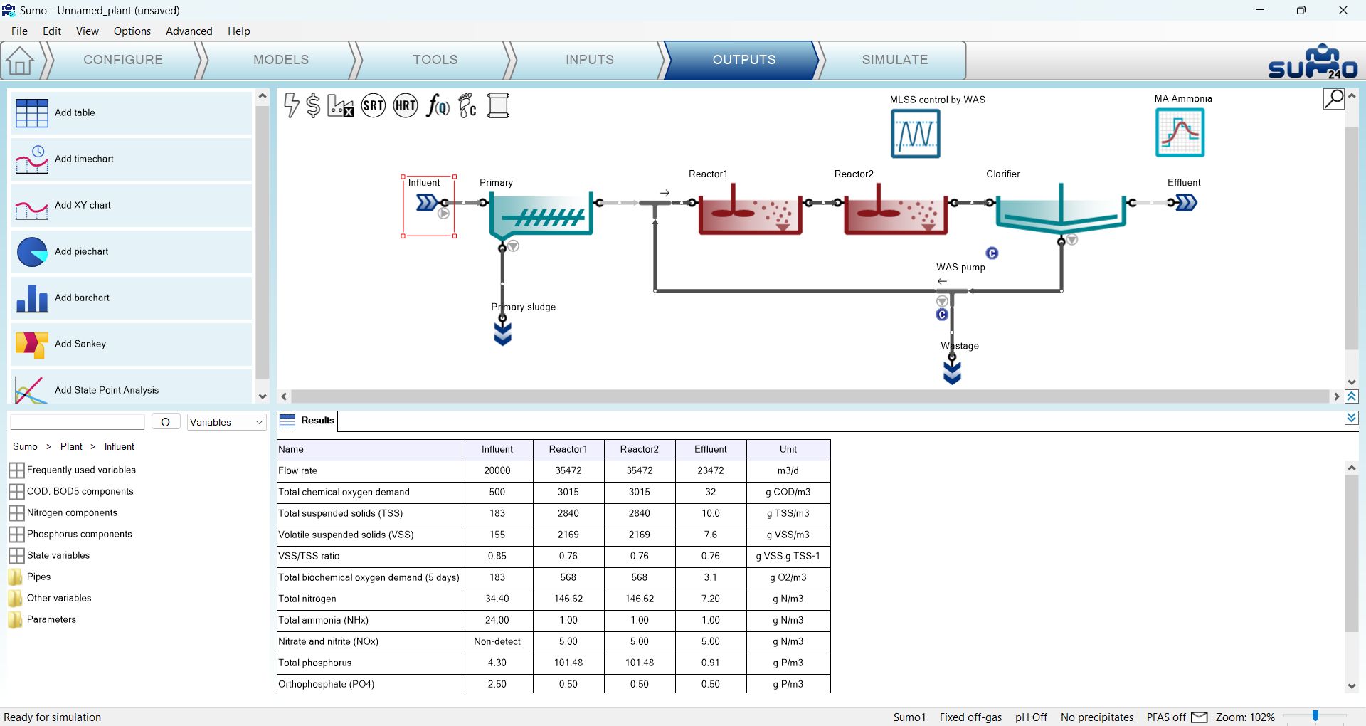
You can add also the DO and Offgas O2 content from the Frequently used variables of Reactor 1 (or 2).
Add another table and drag the Active biomass and Uptake rates for both reactors.
Note that the table columns (except for Name and Unit) can be reorganized by dragging the column header and dropping to the desired slot. Table rows can be rearranged likewise: first highlight the rows to be moved with the mouse, then drag and move the pointer out to the bottom left screen panel for a moment, and finally drop the rows to the desired new place. Units can be changed by clicking and selecting from the dropdown list. The number of decimal digits displayed can be customized to show meaningful detail by hovering the mouse over the numbers and clicking the respective icons – the action will apply to all numbers in the active table row.
¶ Adding a timechart
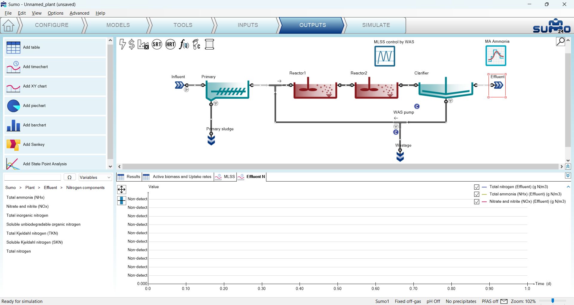
Click the Add timechart button in the top left panel: this will add a timechart to the bottom right panel as a new tab. Select a process unit on the layout and drag a variable from the bottom left panel on the timechart to be plotted (a legend will appear in the top right corner of the timechart). Several variables can be added to each timechart (new items will be appended to the legend), and several timecharts can be added as well (increasing the number of tabs). In this example we will plot MLSS in the reactors and wastage flow on one timechart (select the reactors one by one and add TSS from Frequently used variables); and effluent total nitrogen, ammonia, as well as nitrate and nitrite (available from Nitrogen components) on the second one (see Figure 2.6.3). Graphs will be plotted during the simulation phase.
¶ Adding an X-Y chart
This type of diagram can be used to demonstrate the relation between selected variables (e.g. equilibrium species) depending on another variable (e.g. pH). A practical application is shown in the example called Titration of ammonia solution.
¶ Adding a piechart
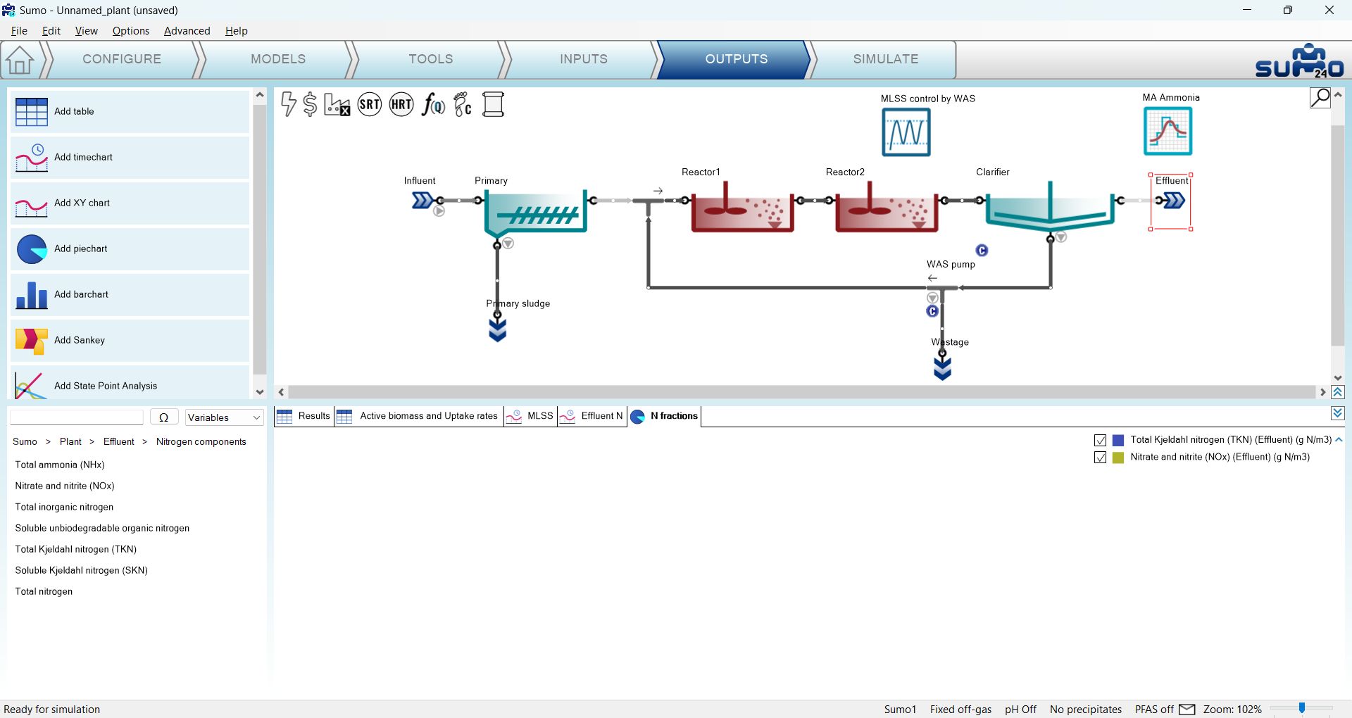
Click the Add piechart button in the top left panel: a new tab for labeled piechart will appear in the bottom right panel. Select the desired process unit on the layout and drag the variables to be depicted from the bottom left panel to the – yet empty – bottom right panel (a legend will appear in the top right corner). For this example, we will use Total Kjeldahl Nitrogen along with Nitrate and nitrite (available from Nitrogen components) in the effluent. Rename the tab to “N fractions” (Figure 2.6.4). The piechart will be rendered during the simulation phase.
¶ Adding a barchart
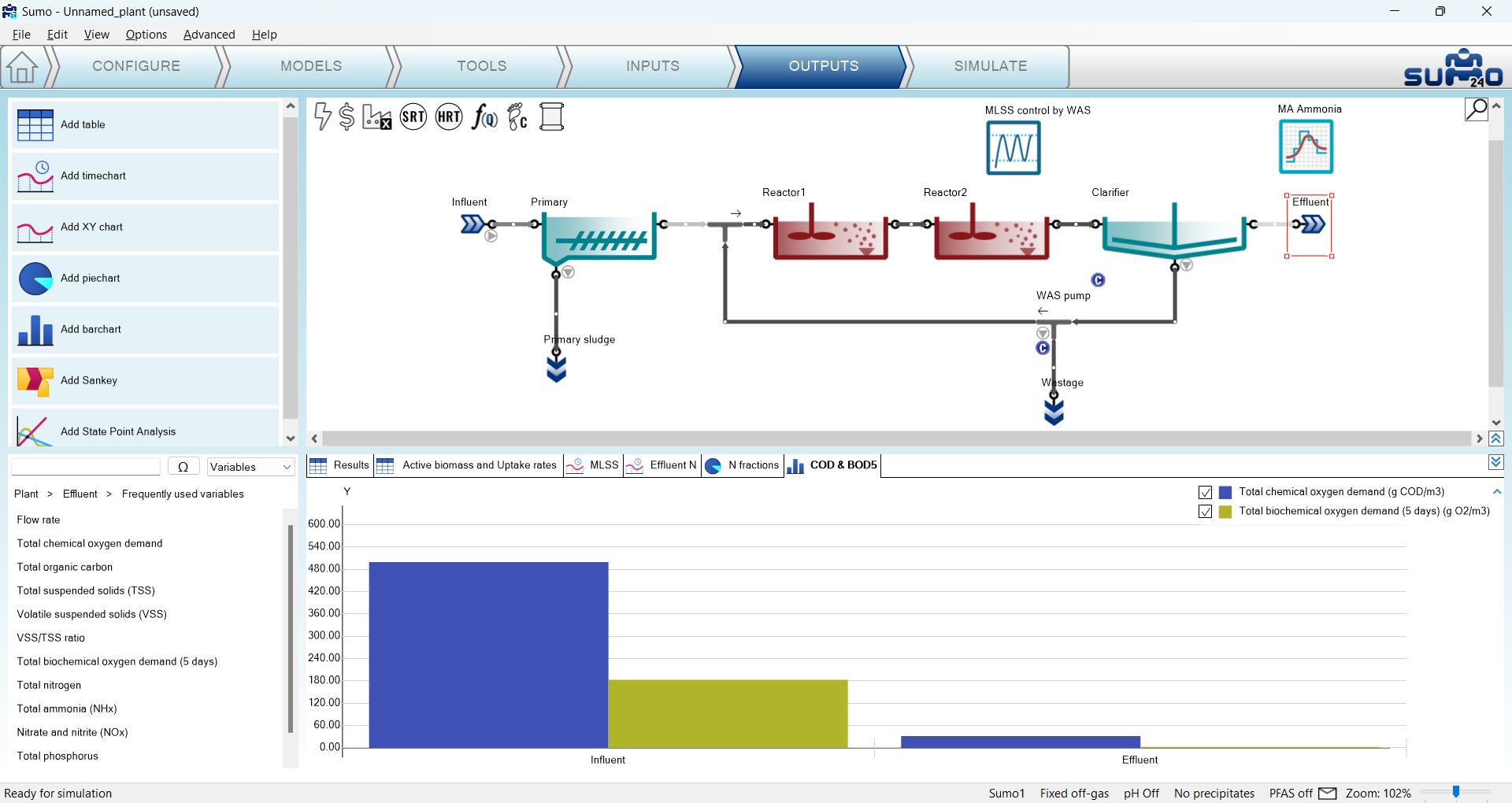
Click the Add barchart button in the top left panel: this will add a barchart to the bottom right panel as a new tab. Choose a process unit and drag variables from the bottom left panel to be shown on the barchart, just like in the previous chart types. Multiple variables can be added to each barchart, and several barcharts can be added as well. Dragging additional process units to the chart will add them with the actual set of variables and initial values will be shown. For this example, choose Total chemical oxygen demand and Total 5-day biochemical oxygen demand from the Frequently used variables in the influent and in the effluent (Figure 2.6.5). Rename the tab as “COD & BOD5”. The barchart will be continuously updated with the changes during the simulation phase.
Note that the order of process units in the barchart can easily be reorganized by dragging the name of the process unit and dropping it to the desired slot.
¶ Adding a Sankey diagram
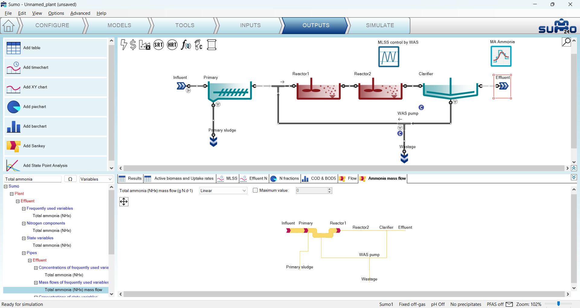
Click the Add Sankey button in the top left panel: this will add the Sankey diagram of flow by default. The variable can be changed by dragging any other item from the bottom left panel over to the bottom right panel. Several Sankey diagrams can be added, with one variable plotted on each Sankey. This example will use one Sankey with the default setting (renamed to “Flow”) and another one showing the mass flows of ammonia (renamed as “Ammonia mass flow”) as shown on Figure 2.6.6. Use the search field in the bottom left panel to find the latter: type in “Total ammonia” and locate “Total Ammonia (NHx) mass flow” under the “Mass flows of frequently used variables” list item in the search results. The search field works with all of the other output options as well.
¶ Adding an SPA chart
Starting with SUMO24, State Point Analysis chart is also part of the Outputs. An SPA diagram is a graphical tool that is used to evaluate the settling characteristics and performance of a clarifier in a wastewater treatment system. This output type requires having a 1D layered clarifier model, so we won't use it in our current simple tutorial plant. For further explanation please refer to the Advanced simulations chapter.
At this point, the example is prepared for simulation with all the inputs and outputs provided. If desired, the output tabs can be reordered by dragging them to the aimed sequence. The file can be saved using the File menu (this function is not available in the demo version).
¶ Simulate
The last item on the Task Bar can be used to run simulations and observe the results.
The role of screen panels in Simulate mode are the following:
| Top right panel | Plant configuration |
| Top left panel |
Simulation control panel Different function buttons for the simulation, including report preparation in Excel format. |
| Bottom right panel |
Tabs for the previously defined outputs Display of results. |
| Bottom left panel | Tabs for scenario definition |
¶ Simulation Control Panel
The top left screen panel enables operating the model by running dynamic or steady-state simulations (Figure 2.7.1). The simulation launchpad offers three modes that can be shuffled by a rotating circular button (hovering over the icons will reveal a descriptive label that helps identifying them). The Steady-state mode (blue circle icon) can be used to calculate directly the steady-state condition of the system, while using the Dynamic mode (red triangle) will show the variations with time, whereas the third, Dynamic from steady-state mode (blue circle with red triangle) will combine the two. The actually selected mode will be positioned on the right side of the circular button, highlighted by a slightly darker background color.
Four additional buttons are placed next to the simulation launchpad. In the top row you can toggle between two pre-configured solver settings: Fast (default) and Accurate, denoted by stopwatch icons. In the bottom row you can find the Reset and Pause/Continue buttons. The latter button will interrupt a running simulation (or resume a previously interrupted one from the point where it was paused), while the former will reinitiate the next simulation with the default concentrations defined in the model and process units. One should use the Reset button thoughtfully, especially when working with complex plants, as reaching steady-state again might be time-consuming (only use it if the goal is to restart the simulation process entirely from scratch).
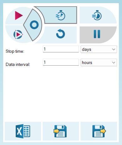
The bottom section of the Simulation control panel consists of three additional button for Generating a report and for Saving and loading plant conditions.
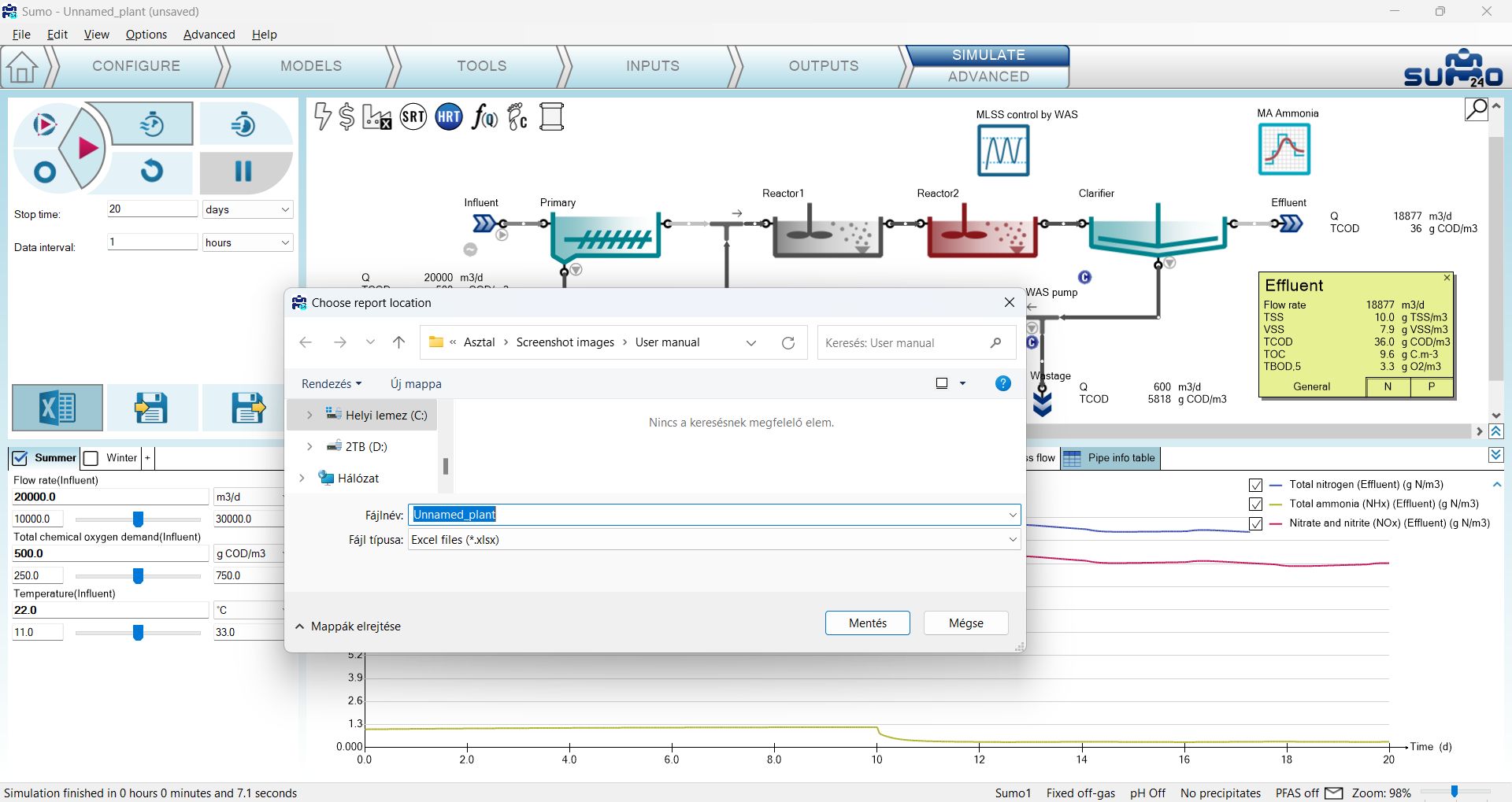
Generating a report with the results of the last simulation is also possible by clicking the spreadsheet icon in the bottom part of the Simulation Control Panel (more on that in the Writing a report section later).
The Save/Load plant conditions functionality can be useful to modify the system state to define the initial conditions for the next simulation. The two disk icons in the bottom part of the Simulation Control Panel (below the Stop time and Data interval fields) serve this purpose. Please note however, that this function is not equivalent to saving the entire project (layout, model setup, tools, inputs and outputs etc.) using the Save/Save as commands in the File menu. More details can be found under the Advanced simulations chapter's Save and Load plant conditions section.
¶ Steady-state simulation
In systems theory, a system or a process is in a steady-state if the variables which describe the behavior of the system or the process do not change with time. If a system is in steady-state, then the recently observed behavior of the system will continue into the future.
After setting up the plant, all process units get a predefined initial value for each state variable (taken from the model defaults). However, most often this will not equal the values that can be observed in steady-state condition. The steady-state calculation will find the proper state variable values when the system is in steady state.
The steady-state simulation employs different solvers to look for the steady-state condition of the system. In this mode, all dynamic inputs are disabled and the controllers are turned into integrated controllers. Please note that steady-state simulation cannot be performed on inherently dynamic processes such as the SBR.
¶ Dynamic simulation
A dynamic simulation will follow changes within the system as time passes, starting from the actual state of the system, and applying all dynamic inputs and behaviors that were defined during the setup process.
Upon the first start after setting up the plant, the simulation will be run from the initial conditions (defaults specified in the model file and in the process units). Every subsequent run will be initiated from the last system state. The actual system state gets saved when saving the project (and additionally, you can save the current system state anytime using the dedicated disk icons of the Simulation Control Panel, as described above).
The dynamic simulation will run until the end of the period defined by Stop time is reached (default setting: 1 day) and will plot/update results in the bottom right screen panel with the frequency described by the Data interval (default setting: 1 hour). The Stop time and Data interval can be modified on the Simulation Control Panel before the simulation is started, and also when it is paused.
¶ Dynamic simulation from Steady-state
This mode performs a steady-state simulation prior to starting a dynamic one. Use it if the dynamic simulation with the prescribed Stop time and Data interval should start from steady-state.
¶ Fast and Accurate solver settings
Choosing between Fast and Accurate switches to either of the two pre-configured solver settings. The differences between these are described in Table 2.7.1. Usually the Fast mode is fast and accurate enough for most cases, and therefore its use is generally recommended. However, in certain situations (e.g. with biofilm models), the Accurate mode might provide faster simulation. If the plant seems to be complex and takes a long time to find a solution in Fast mode, then try switching over to Accurate. In such rare cases, it is the trial-and-error of coming to solver settings that lead to a speedy solution. There is no difference in the stop criteria for the solvers.
Table 2.7.1 – Explanation of Fast and Accurate solver settings
| Fast | Accurate | |
| Type of configuration | Simple plant layouts will provide a speedy simulation | Best for complex plant layouts, specifically which have biofilm processes (MBBRs, and trickling filters) and several return or recycle streams. |
| Solver types | GISA → Relaxation solver → Newton-Raphson | Relaxation solver → Newton-Raphson |
Please note that the mode selection will also have effect on the steady-state solver: GISA introduces a strong perturbance to the system state, therefore it is quite suitable for finding steady-state from a distant initial system state, while not so necessary when the system is already close to steady-state.
¶ A process simulation example – aerobic plant
The plant configuration we have just built is an aerobic plant, with 12-hour hydraulic residence time:

Plant HRT can also be calculated by SUMO, using the Hydraulic Residence Time tool on the Tools tab. Just simply drag the reactors that contain reactive liquid volume to the numerator and drag the influent unit in the denominator, as illustrated by Figure 2.7.2. Several HRT calculations can be set up, e.g. total, anoxic, aerobic, or HRT of one of the parallel trains, etc. When the influent flow is split into multiple parallel trains, the respective flow into the designated reactor (without considering recirculation flows) can be defined by multiplication of the overall influent flow and a ratio parameter (which is available in the Inputs tab, selecting the HRT icon). Note: when the project has an HRT calculation set up, the HRT icon on top of the drawing board gets a blue color.

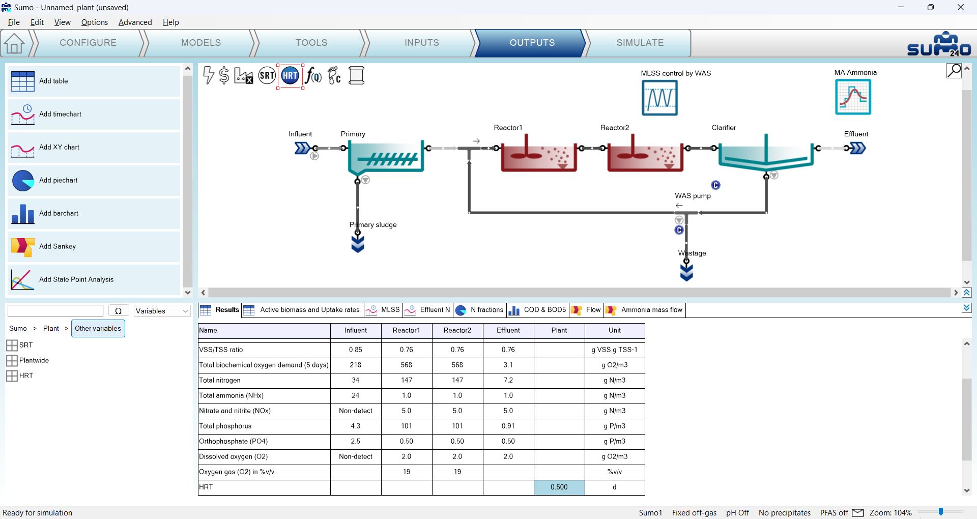
After having set up the HRT calculation, move back to the Outputs tab and while SUMO recompiles the plant (this will happen every time you change something on the Configure, Models or Tools tab and return to the Inputs, Outputs or Simulate tab), select the HRT icon and in the bottom left window pane navigate the output options to Sumo>Plant>Other variables, then add HRT to the Results table in order to show the plant HRT calculated by SUMO (Figure 2.7.3).
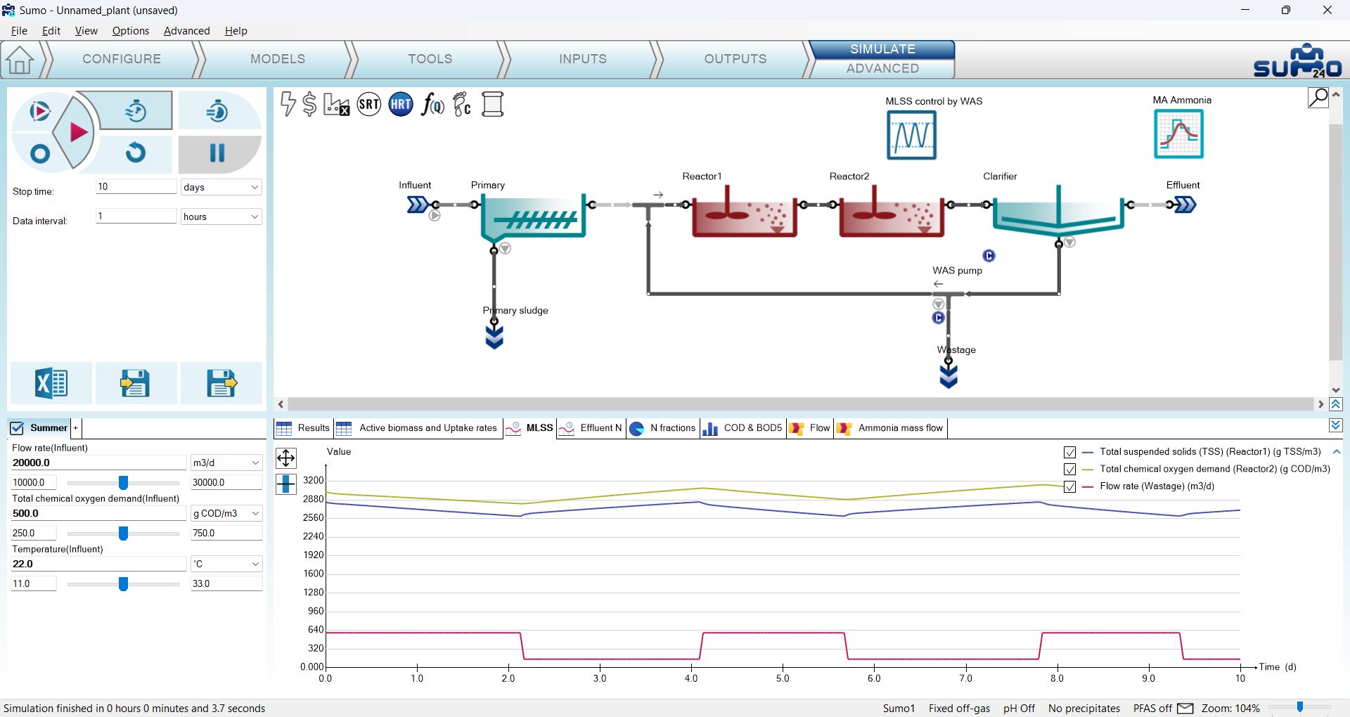
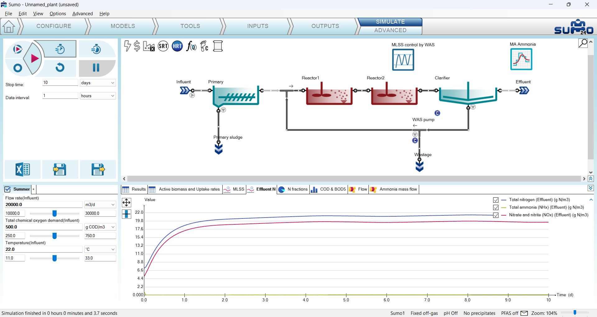
Now it's time to move to the Simulate tab and start simulations. A 10-day MLSS graph gives a good indication whether the system has settled into stable condition and the results are meaningful for typical dry weather summer operation, so let us start by setting the stop time to 10 days with 1-hour data interval and running a dynamic simulation. MLSS and effluent N plots are presented by Figure 2.7.4 and Figure 2.7.5, respectively. The effect of the MLSS control strategy can be observed as well.
In the bottom left screen panel rename the Default scenario to Summer (in order to differentiate from an another scenario that will be added later on).
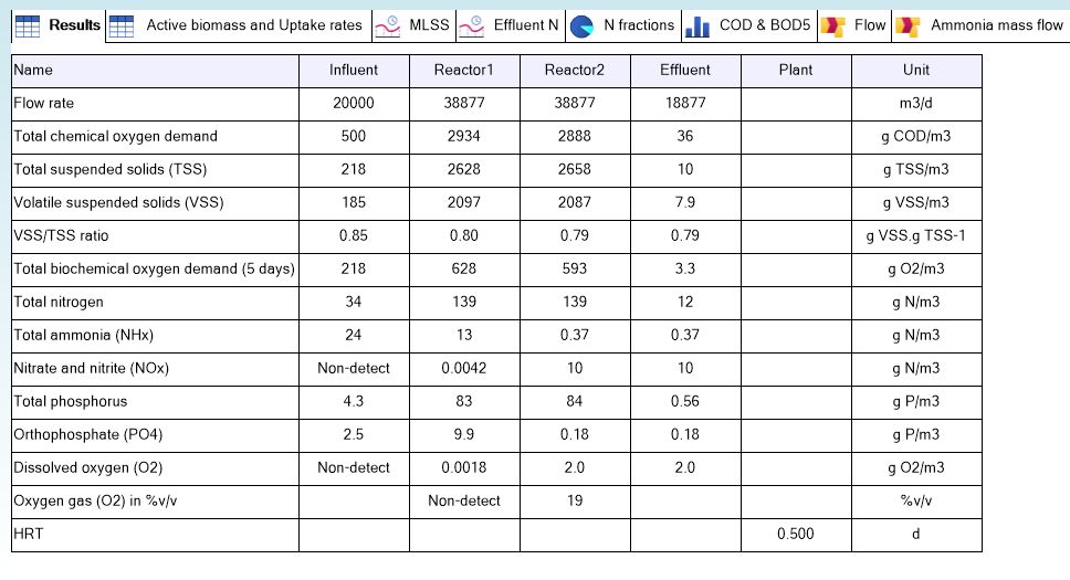
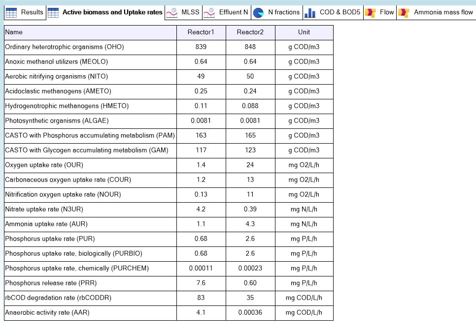
The tabular results are shown in Figure 2.7.6 and Figure 2.7.7.
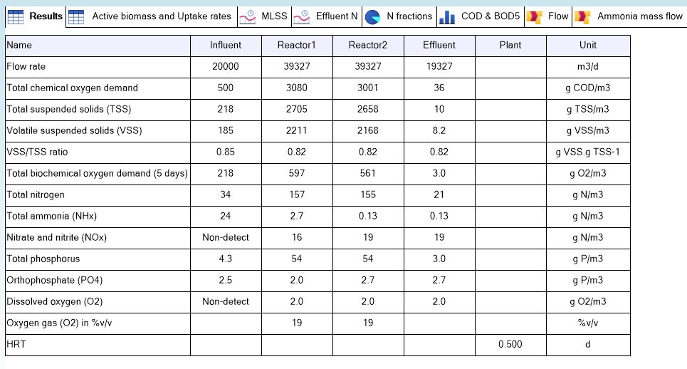
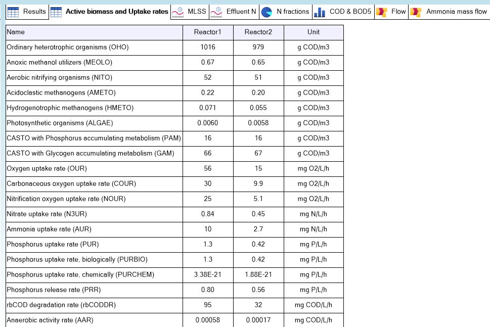
These tables show:
- TSS and VSS profile from the influent through the reactors to the effluent;
- High effluent nitrate and low effluent ammonia (full nitrification);
- DO of 2 mg/L in both reactors (due to input settings);
- Oxygen Uptake Rate (OUR) in the two reactors: higher in the first one, lower in the second, as expected.
This fully aerobic plant does nitrify completely, producing low ammonia and high nitrate concentrations in the effluent. Both reactors are aerated to 2 mg/L DO, which requires energy and comes with costs.
¶ Implementing denitrification
In the system above, the main electron acceptor for biochemical reactions is dissolved oxygen. We can use the abundant nitrate as electron acceptor, and with this process reduce our energy requirement and improve the effluent quality at the same time. For this, we need to reconfigure the plant – in this case simply creating an anoxic zone by switching off the aeration in Reactor 1. (In the actual plant, mixers would need to be installed in the anoxic zone to keep the MLSS in suspension, but in the model, the reactors are always ideally mixed.)
To implement this change, select Inputs on the Task Bar, switch to Constants mode, select Reactor 1 and select the Aeration settings item from the Input parameters (bottom left panel), then change the DO setpoint to zero in the bottom right panel (Figure 2.7.8).
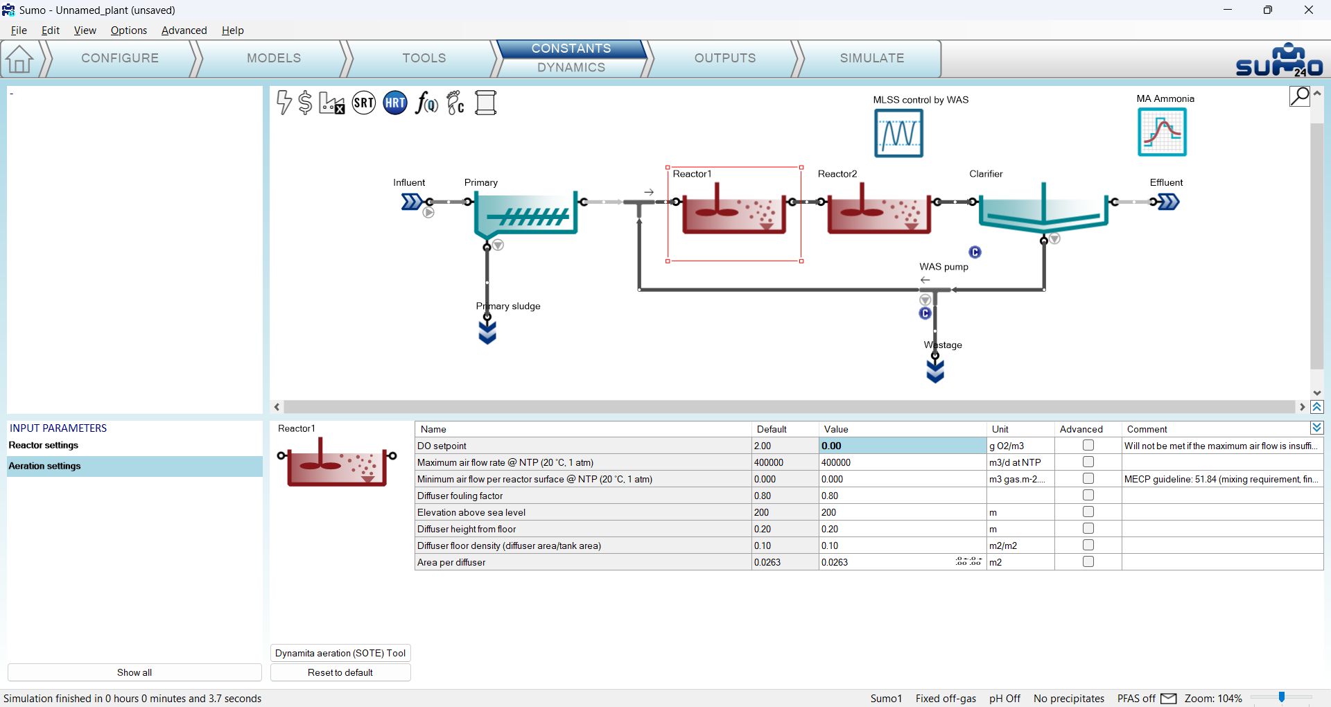
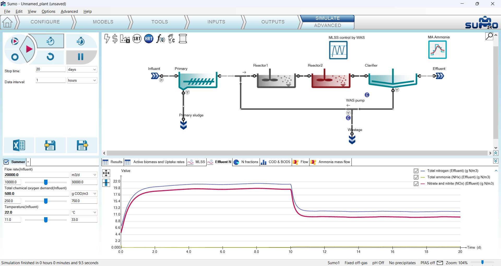
Go back to the Simulate tab, set the Stop time to 20 day and click Continue (note that the Pause button will turn to a red triangle when you set the stop time to a larger value than the previous setting). The simulation will go on while keeping the results of the previous 10 days in the graphs. Note that the color of the first tank will change to grey: this feature serves for easier visual identification of anoxic/anaerobic reactors. The effluent nitrate will be reduced because it is used up to oxidize organic material in Reactor 1 (the anoxic zone). On the contrary, effluent ammonia increases slightly as nitrification requires aerobic conditions and the aerobic reactor volume was reduced from 10000 m3 to 8000 m3. The effect of the DO setpoint change in the Reactor 1 can be followed in Figure 2.7.9. The drop in effluent nitrate concentration after 10 days is a due to the Reactor 1 having been turned anoxic. The time frame of the change can be followed as well: within 24 hours the nitrate concentration drops to the lower value.


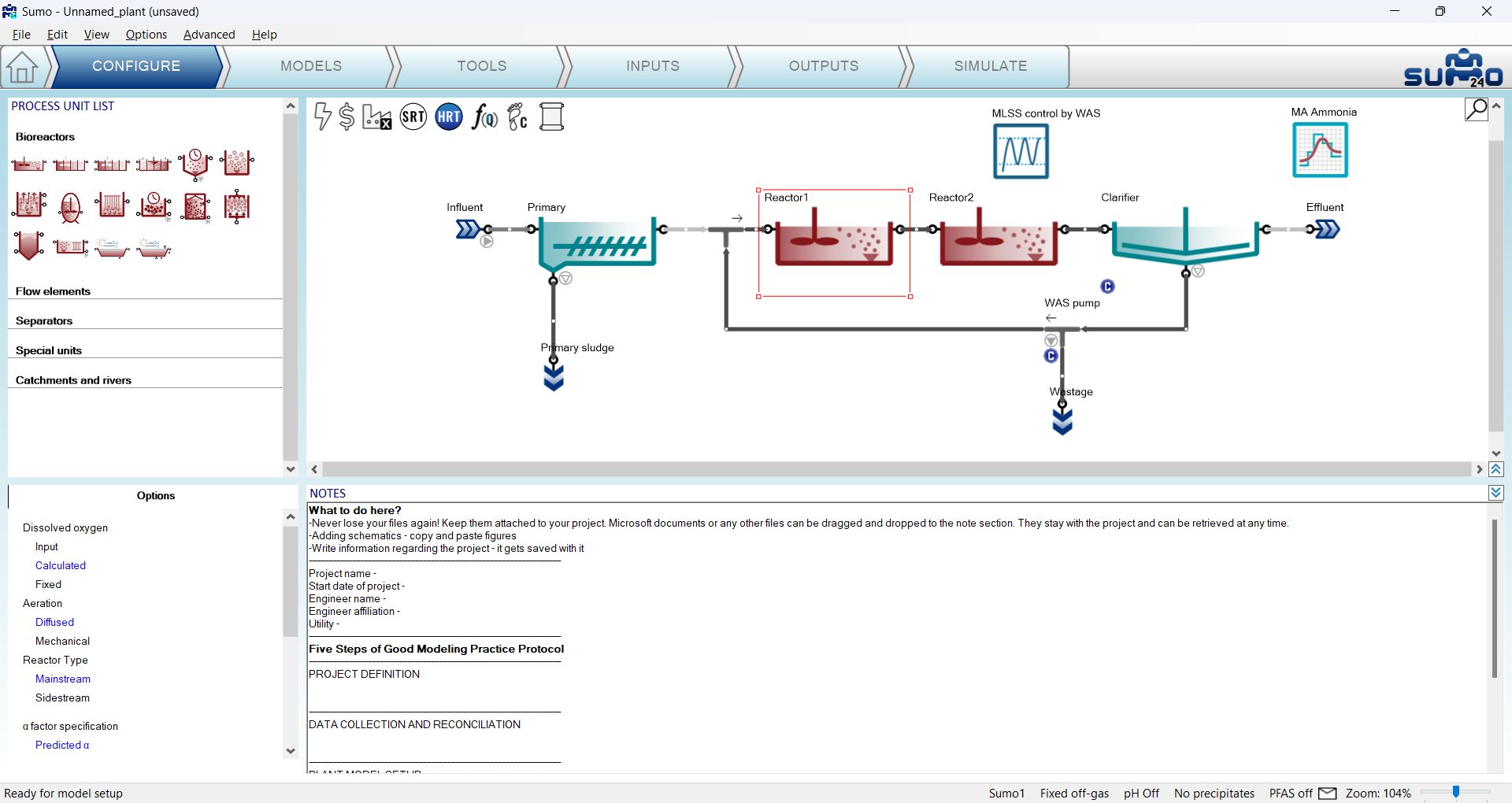
Besides calculating air flow from a defined input DO, Sumo also offers the possibility to calculate DO levels based on specified input air flow. To select this model option, go back to the Configure tab and select Reactor 1, then in the Dissolved oxygen process unit option, switch from Input to Calculated (Figure 2.7.12). The calculated DO option will provide a better estimate of expected effluent values. In an aerobic reactor, instead of DO setpoint, the air flow is defined in the Inputs, and the concentration of the DO is calculated based on a mass transfer model. In anoxic (and anaerobic) reactors, with zero airflow specified, only the DO introduced by their input flow is considered.
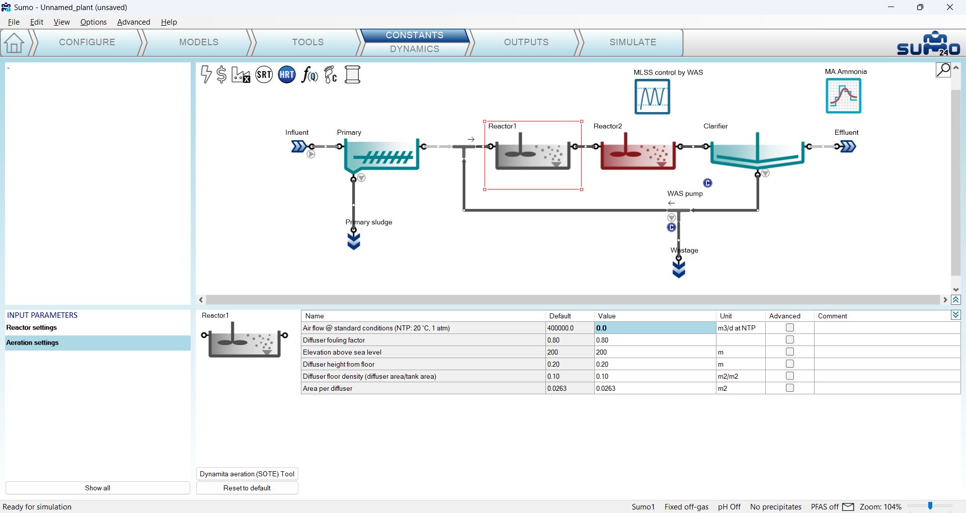
The air flow can be provided on the Inputs tab. Let us change the blower airflow of Reactor 1 to 0 (Figure 2.7.13):
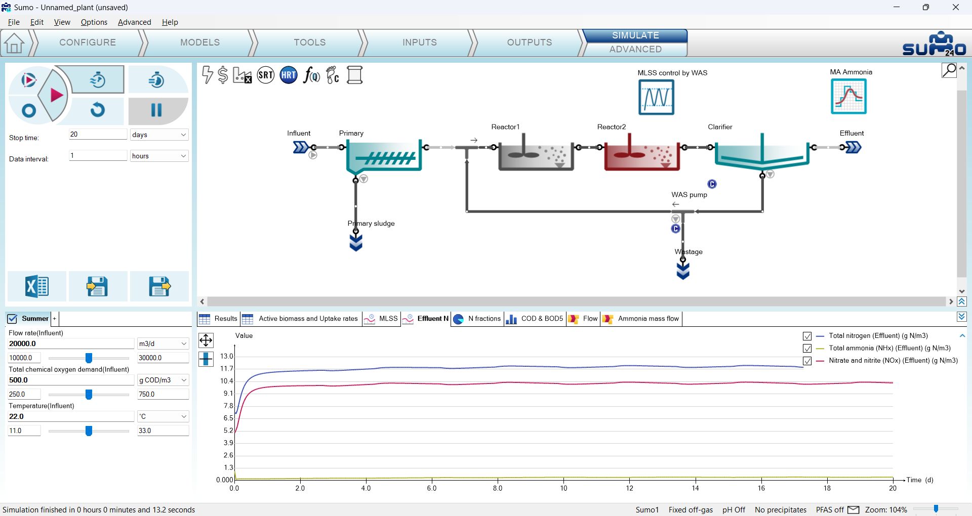
After clicking on Reset, then running a 20-day simulation, you can compare the results of the plant operating with input DO (Figure 2.7.9, Figure 2.7.10 and Figure 2.7.11) and the plant operating with calculated DO (Figure 2.7.14, Figure 2.7.15 and Figure 2.7.16):
¶ Subjecting the plant to dynamics
Plants are usually subjected to diurnal variation and we might be interested not only in the average, but the peak effluent concentrations as well (e.g. in certain jurisdictions the effluent limits are based on grab samples never to exceed, daily maximum, etc.). This requires a dynamic simulation to investigate potential peaks during the day.
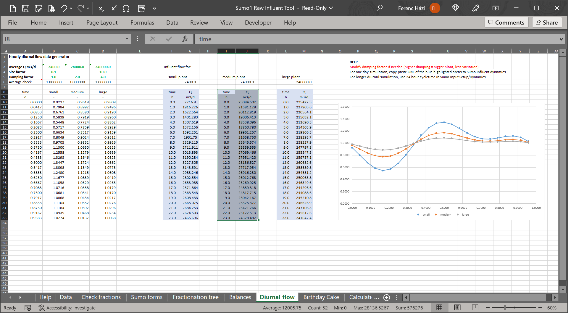
Select the Inputs tab, and the Influent process unit, where we are going to provide diurnal flow variation. In Constants mode, the Influent tool is available for Sumo models as an Excel file, containing typical fractions and diurnal variations with different plant sizes. Click on the button (located in the bottom right screen panel) to open this tool and copy the “medium plant” table from the Diurnal flow sheet to the clipboard (Figure 2.7.17):
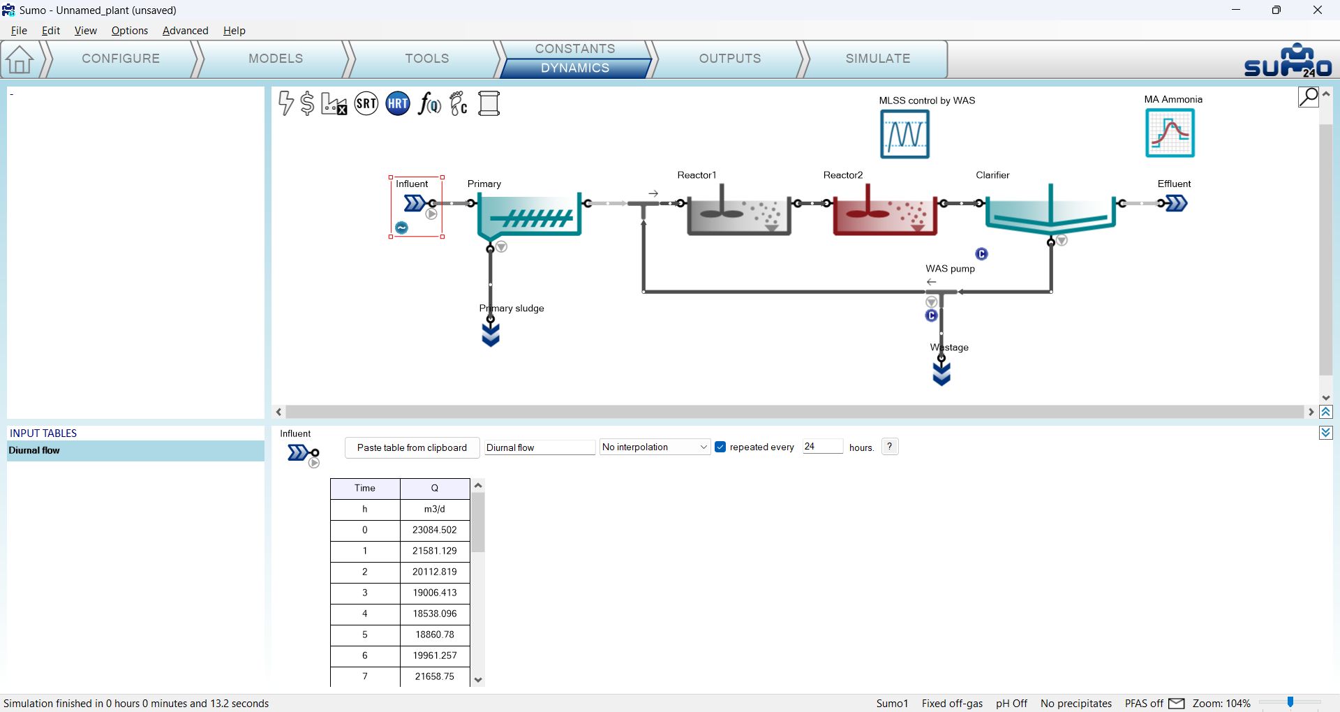
Now switch to Dynamics mode in Sumo and paste your table by clicking on the Paste table form clipboard button (after this, you can close the Influent tool Excel file). On the drawing board, a small sign will appear below the Influent, showing that dynamic parameter input is used. These tables can be disabled/enabled or deleted by right-clicking on the name in the bottom left screen panel. Note that for a certain variable/parameter, only one dynamic table can remain enabled (Sumo will give you a warning if more than one tables are enabled for the same subject). The names of disabled tables (which are editable in the bottom right screen panel) will show up in grey, and in case all dynamic input tables are disabled, the sign beside the process unit will also turn to grey (indicating that there are dynamic inputs available, but not used). Linear interpolation and cycle repeat can also be set for dynamic input tables. Rename the newly inserted dynamic input table in the example to “Diurnal flow”, check the box to repeat the contents of the table and provide the repeat frequency as 24 hours in this example, as depicted on Figure 2.7.18.
If you can provide data from measurement, your input data (flow variation in this case) should be in Excel, in the following format: the header should be “Time” (“time” is also accepted) and the selected variable name as it is used by Sumo, in this case “Q” (denoting flow), with the respective units (“h” and “m3/d”) in the second row, as illustrated by Table 2.7.2.
Table 2.7.2 – Dynamic input of influent flow pattern
|
time |
Q |
|---|---|
|
h |
m3/d |
|
0.0 |
23084.502 |
|
1.0 |
21581.129 |
|
2.0 |
20112.819 |
|
3.0 |
19006.413 |
|
4.0 |
18538.096 |
|
5.0 |
18860.780 |
|
6.0 |
19961.257 |
|
7.0 |
21658.750 |
|
8.0 |
23645.574 |
|
9.0 |
25559.553 |
|
10.0 |
27069.466 |
|
11.0 |
27951.420 |
|
12.0 |
28136.527 |
|
13.0 |
27717.954 |
|
14.0 |
26916.230 |
|
15.0 |
26012.768 |
|
16.0 |
25269.925 |
|
17.0 |
24859.318 |
|
18.0 |
24817.715 |
|
19.0 |
25042.167 |
|
20.0 |
25325.377 |
|
21.0 |
25421.266 |
|
22.0 |
25122.513 |
|
23.0 |
24328.482 |
To find out what is the internal identifier for a certain variable (or model parameter), you can just hover the mouse above the name of the specific item in the parameter tables of Inputs – Constants (or in the case of model parameters, the Models), and a popup will show you the cryptic name of your input variable that has to be used in the dynamic table (see Figure 2.7.19). For your comfort, right-clicking here offers an option to copy this symbol directly to the clipboard (and the same goes for units), from where you can paste it into your table.
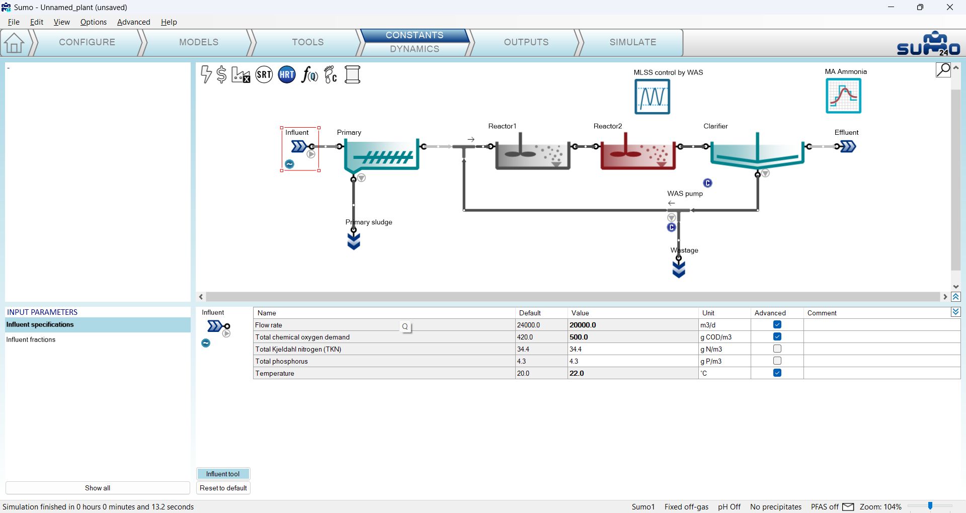
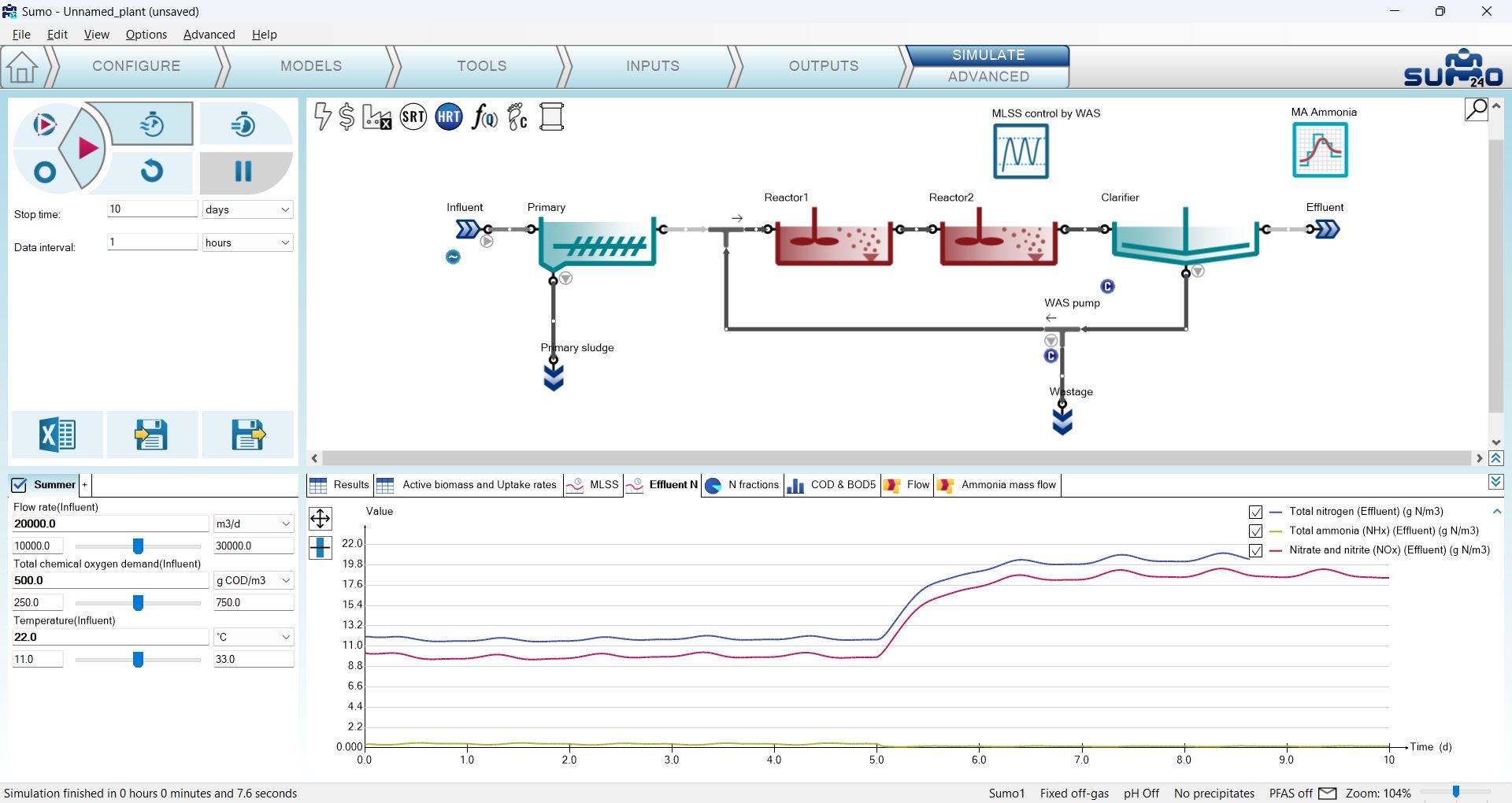
Having set up the diurnal flow, go to the Simulate tab and start a new dynamic simulation of 5 days duration: In this case, the result of the last simulation will be used as initial values. The variation in loading should have an effect on effluent quality, as shown by Figure 2.7.20.

We can observe higher ammonia concentrations during the high loaded periods, and lower nitrate concentrations, due to lower nitrification and the abundance of organic substrate for denitrification.
We can of course always turn on our aerators in the first reactor (not so easy in an actual plant) by going to the Inputs tab, selecting Reactor 1 and changing the air flow to 150000 Nm3/d. In the Simulate tab, we can extend the length of the run for 10 days and hit Continue.
Nitrate concentration will increase, and the ammonia peaks will get much reduced from day 5, when the aerators were turned back on. After this exercise, reset the air flow in Reactor 1 to 0 Nm3/d and run a 10 d simulation to get back to denitrifying plant.
¶ Model parameter dynamic input
Model parameters and plantwide parameters can be added as dynamic inputs as well – in these cases, the plantwide (factory) icon should be selected on the drawing board in the Inputs – Dynamics tab, and the extended incode names of the model parameters are to be used in the dynamic input tables, as described below.
The incode name of model parameters can be found as popup by hovering the mouse over the desired parameter on the Models tab. See the example of Maximum specific growth rate of the NITOs (nitrifier organisms) on Figure 2.7.22: µNITO is the name of the parameter in the active model, which is the Sumo1 model in this tutorial. A right-click with the mouse enables you to simply copy the name, just like in the case of process unit parameters.
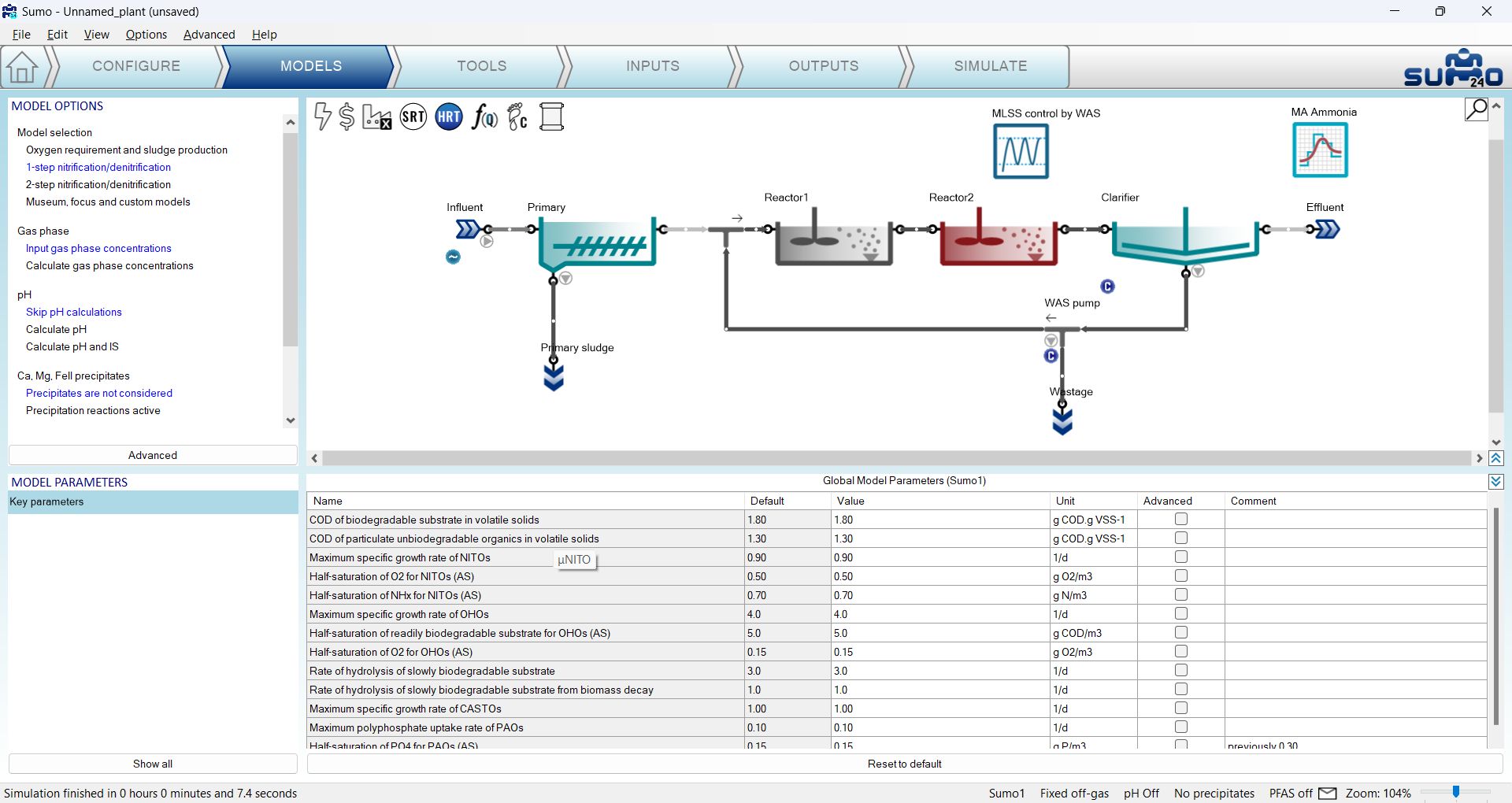
The name to be used in the dynamic input table is the compound of the model name and the parameter incode name, separated by two dots. So in our example, Sumo1..µNITO will be the correct model parameter name to be used (Table 2.7.3).
Table 2.7.3 – Model parameter dynamic input table
|
time |
Sumo1..µNITO |
|
h |
1/d |
|
0.0 |
0.9 |
|
6.0 |
0.4 |
Inserting the dynamic input table is done the same way as it was done in the diurnal flow – just copy the prepared table from Excel and paste using the button in the Inputs – Dynamics tab (remember that the factory icon shall be selected for showing this functionality). The presence of the dynamic global model parameter input will be indicated by a blue circle with a wave inside on the drawing board, below the factory icon (see Figure 2.7.23).
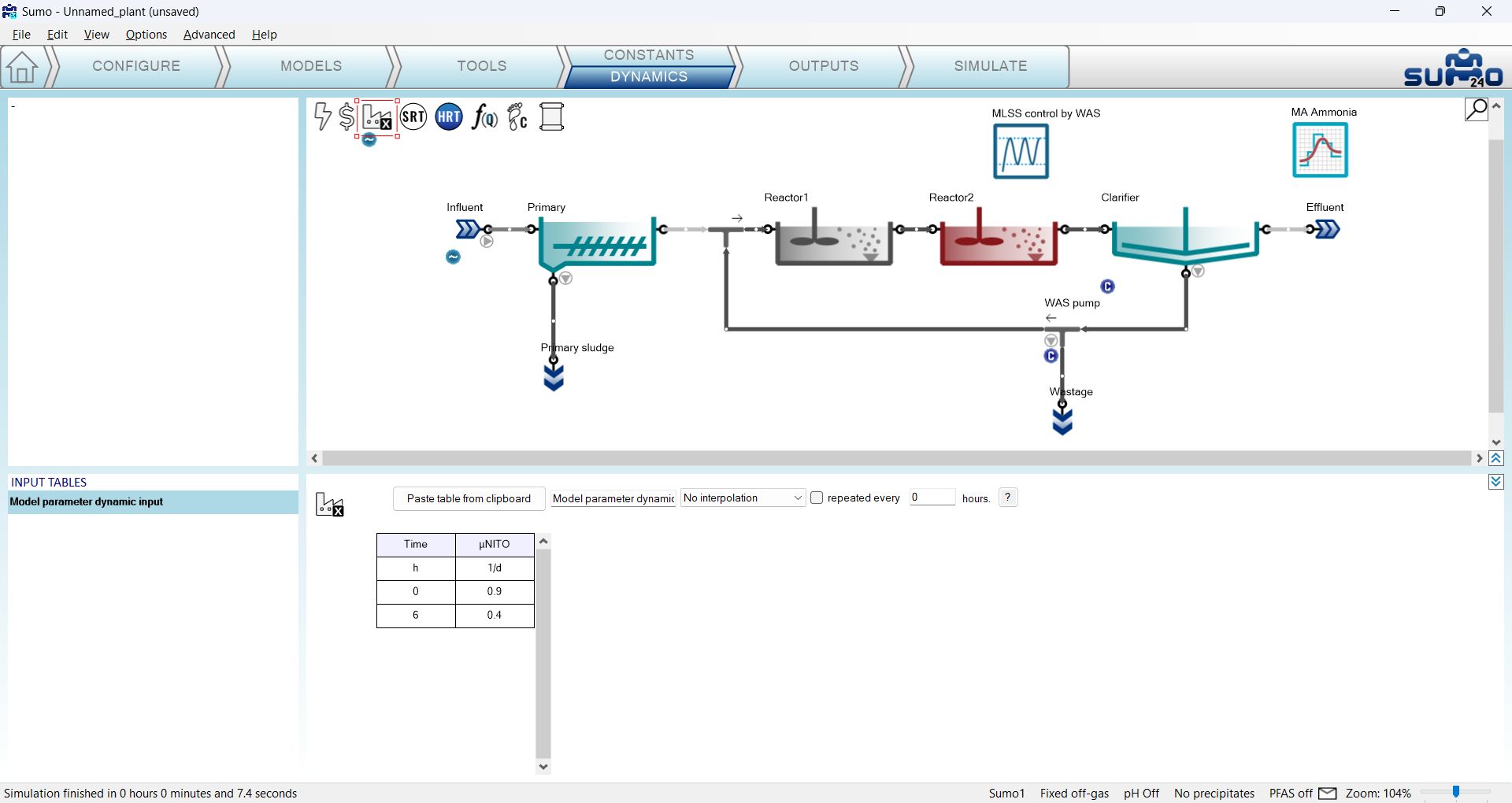
Now let us go to the Simulate tab and start a 2-day dynamic simulation with an hourly data interval. The decrease in nitrifier maximum growth rate (caused by i.e. a toxic substance in the influent) should have an effect on effluent quality as shown in Figure 2.7.24: we can observe higher ammonia concentrations after the decrease in the NITO growth rate.

During the following exercises, we will not use the dynamic input for model parameters any more. In the bottom left screen panel of the Inputs/Dynamics tab, right click on the name of this table and choose Delete table to remove the table. Alternatively, you can just use the Disable table option as well, in order to keep the table but not to use it during the subsequent simulation. Let us try this option for switching off the diurnal flow (the indicator below the Influent icon will turn to light grey).
¶ Adding measured data to outputs
Plants do collect information and one important task in process simulation is to compare measured data with simulation results (and potentially using the information to calibrate the model).
¶ Adding measured data to table
Measured data can be added to tables at the Output setup. To import data to a table, the data has to be in the right format to match the output setup. The best approach is to build the table with the model output, switch to Symbol identifier (Advanced|Variable identifier|Symbol) and use the report feature to export the required data format - no need to run the simulation, this step is used to generate the Symbols and units in an easy was for data input. The next step is using adding the measured data to the table with properly named column headers. Multiple columns can be added, this example highlight the effluent measurements in Table 2.7.3. for the example plant.
Table 2.7.3 – Measured data for the example plant
| Symbol | Effluent | Unit |
| TCOD | 35 | g COD/m3 |
| XTSS | 10 | g TSS/m3 |
| XVSS | 8.1 | g VSS/m3 |
| TBOD_5 | 3 | g O2/m3 |
| TN | 21 | g N/m3 |
| SNHx | 0.34 | g N/m3 |
| SNOx | 19.6 | g N/m3 |
| TP | 2.8 | g P/m3 |
| SPO4 | 2.6 | g P/m3 |
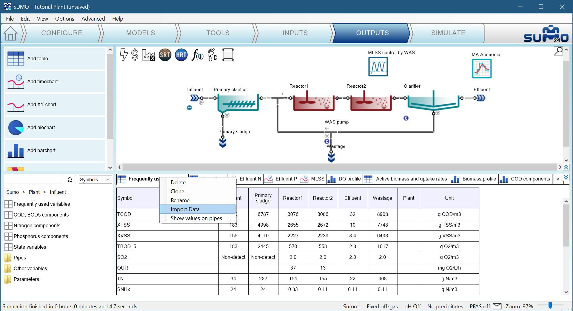
Once the data is ready in the right format copy it and go to the Output setup tab in SUMO, select the table with the relevant variables and from the right-click menu on the tab header select Import data:
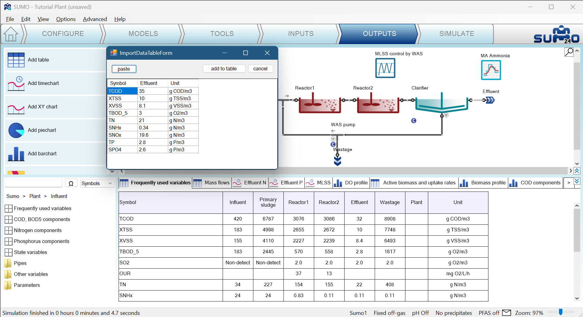
The import data window will be opened and by clicking the ‘paste’ button the data table will be read into SUMO:
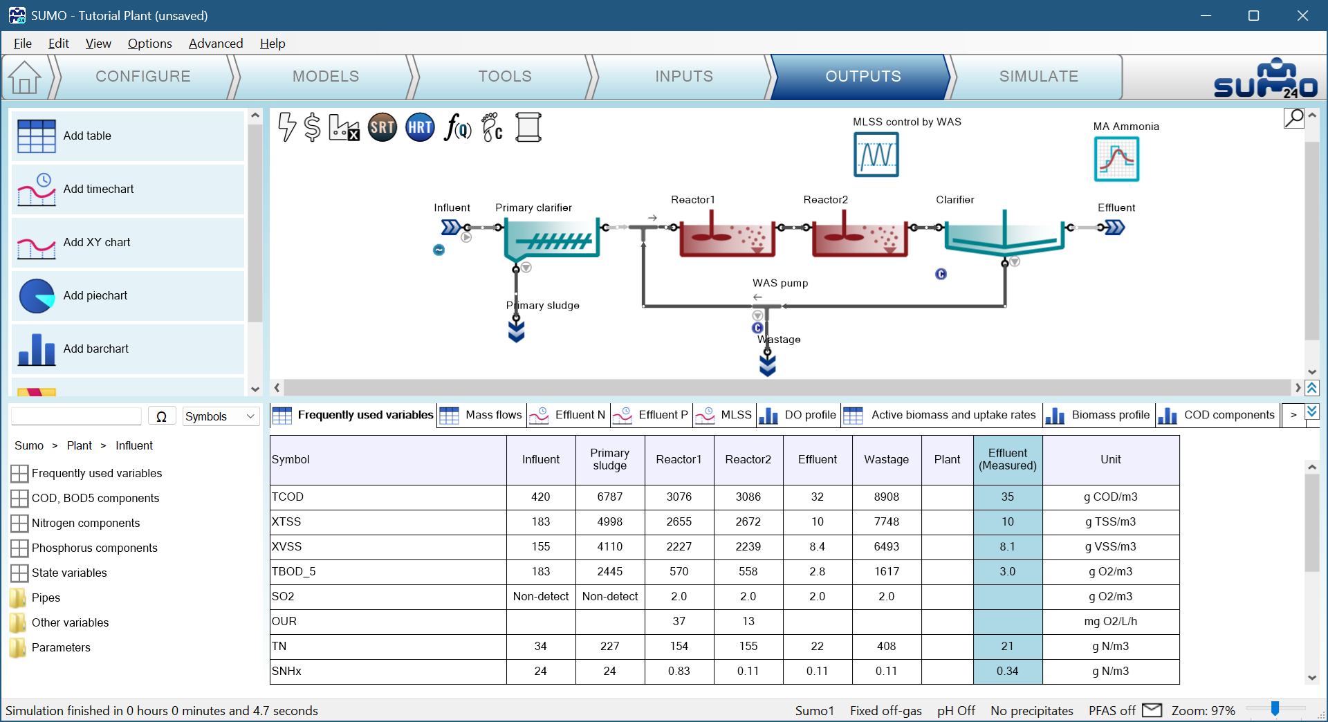
The ‘add to table’ item extends the table in SUMO with the Effluent (Measured) column:
Note: In case of invalid headers SUMO will send a warning highlighting the issue. If there is ‘symbol’ or ‘unit’ mismatch a new row will be added to the table showing the measured value.
¶ Adding measured data to timechart
Let us assume that this plant has MLSS grab samples once a day in Reactor 2 (TSS Reactor 2). The collected data is shown in Table 2.7.5 below.
Table 2.7.5 – Measured TSS data for the example plant
|
Time |
XTSS (Reactor2) |
|
d |
g/m3 |
|
0 |
2800 |
|
1 |
2700 |
|
2 |
2600 |
|
3 |
2700 |
|
4 |
2780 |
|
5 |
2700 |
|
6 |
2750 |
|
7 |
2725 |
|
8 |
2775 |
|
9 |
2600 |
|
10 |
2750 |
Copy this table into an Excel sheet (e.g. named Plant Data.xlsx) and rename the sheet “Measured TSS” (Actual names are irrelevant and flexible).
Now switch to Simulate mode, click on Reset, then run a 10-day simulation to let the system settle into stable condition. Then run another 10-day simulation for evaluating the MLSS trend due to the deadband controller.
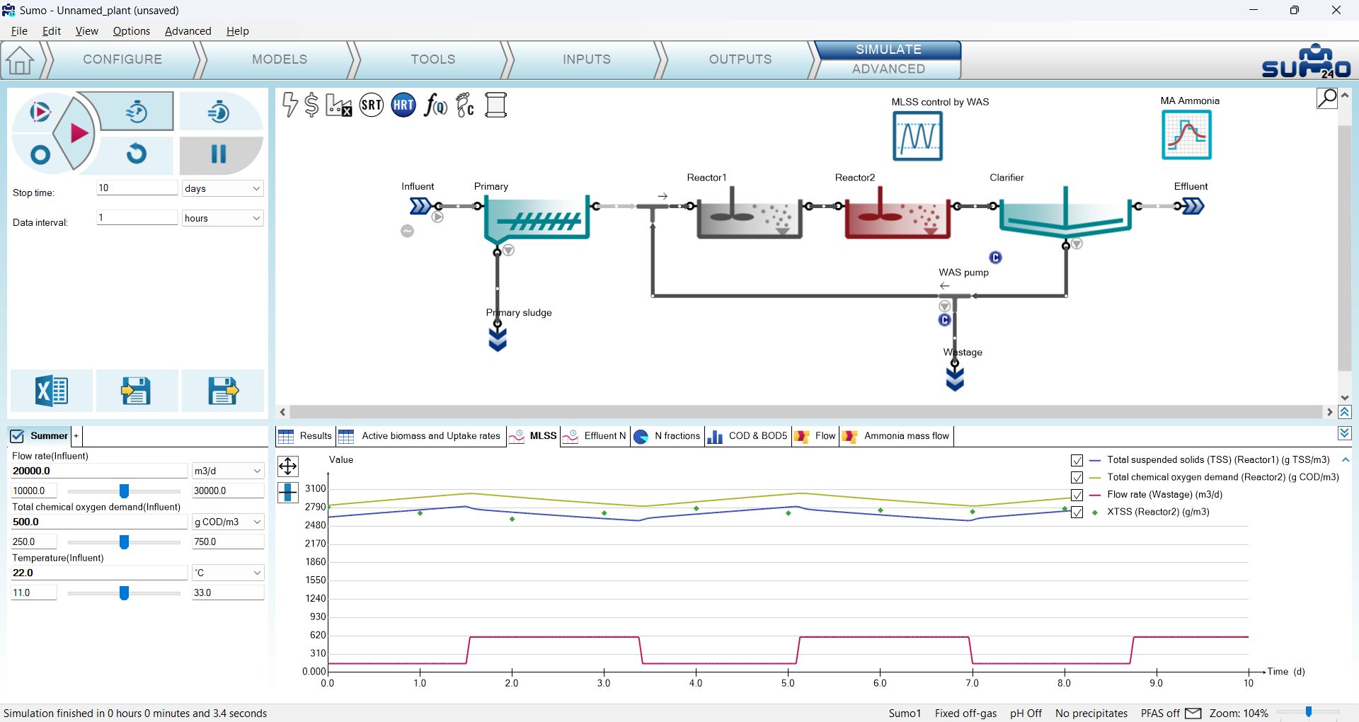
Switch back to Outputs mode, right-click on the MLSS timechart tab and select Import data. The data import is carried out the same way as the dynamic input table: simply paste from the clipboard (Figure 2.7.25).
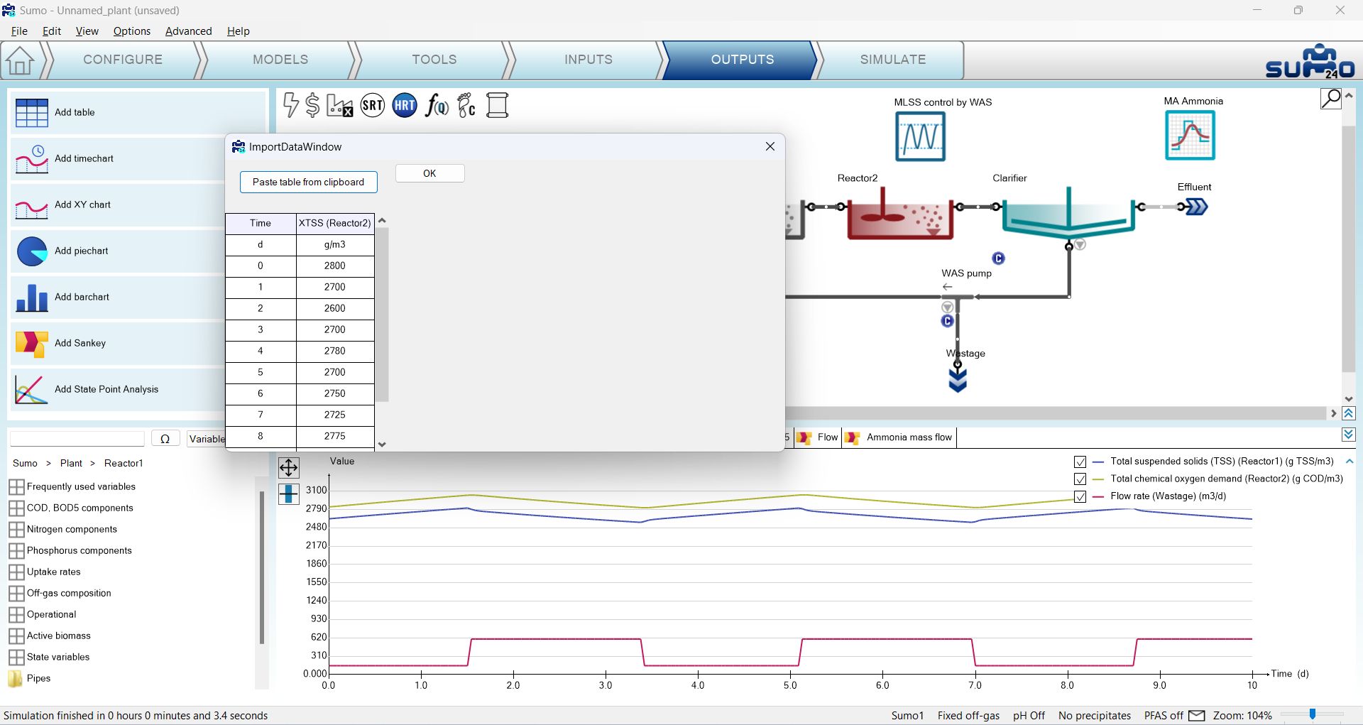
Pressing OK will plot the data along the simulation results (Figure 2.7.26):
The project can be saved any time during the configuration and project development using the File menu and reloaded at a later point in time to continue the work.
Many other operational scenarios can be simulated with Sumo, including more complex reactor configurations and more elaborate operational scenarios. Please see the examples on the Welcome screen and for further description check out the Examples chapter of this manual.
¶ Scenario runs
By default, the simulation is using the input parameters defined in Inputs, such as the influent flow rate, the influent total COD and the influent temperature, which we have also selected for advanced simulation mode at an earlier stage, and renamed the default scenario to Summer. On the bottom left screen panel of the Simulate tab, these parameters are shortlisted. Underneath their name, there is a textbox with their current value (which can be edited directly) and their unit (alternatives are available from a dropdown list). Below these, you will find a slider bar with two textboxes on the left and right hand side, which define the low and high end of the parameter slider (these can be edited as well in order to update the range of the slider). The slider provides another method for changing the value of the parameter. For now we will not change any of these settings for the Summer scenario.
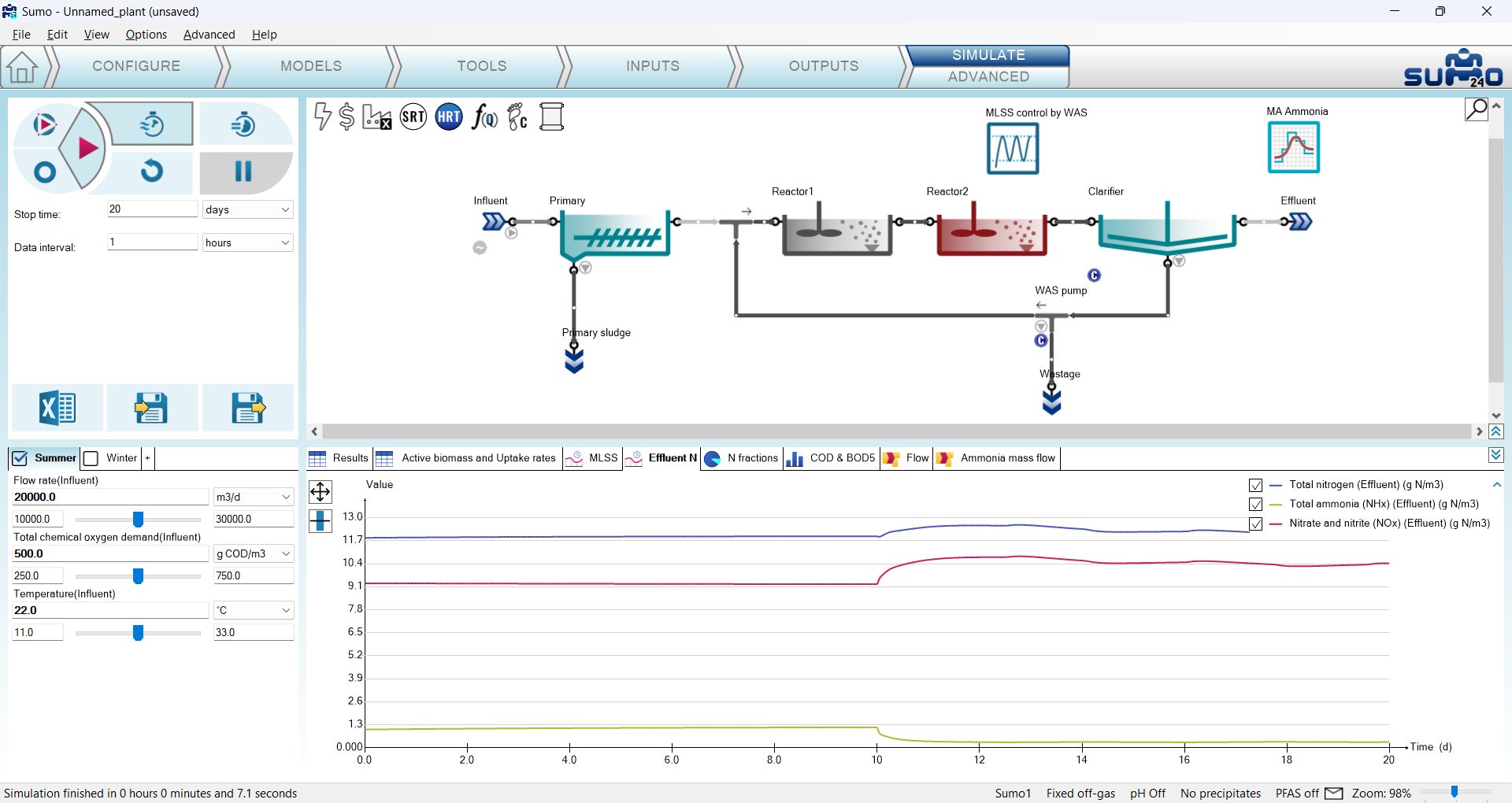
Further scenarios can be defined by clicking on the Add Scenario (+) tab (right next to the last scenario tab). Add a new scenario, rename it to Winter and set 14°C temperature, 26000 m3/d flow rate and 460 mg O2/l total COD as input parameters instead of the default parameter set, then deselect the Summer scenario tab (removing the checkmark) and select the Winter tab in order to activate it for simulation (Figure 2.7.27). With this simple setup, as long as the Winter scenario tab is the only selected one, the simulation will now use 14°C as influent wastewater temperature, modified influent flow and COD composition and the results can be compared. The role of selecting multiple scenarios for a simulation is a new functionality introduced with SUMO24 and will be described in the subsequent Advanced simulations chapter.

After clicking on Reset and running two consecutive 10-day dynamic simulations (in order to get the system to a characteristic winter operation), activate the Summer scenario by selecting its tab (along with deselecting the Winter scenario tab), modify the simulation stop time to 20 day and hit Continue. The change due to new influent conditions can be seen quickly (Figure 2.7.28):
If you want to add further parameters, just go back to the Inputs tab and select the desired parameters of the desired process unit. Model parameters can be selected as well for scenario runs from the Models tab.
¶ Adding popups
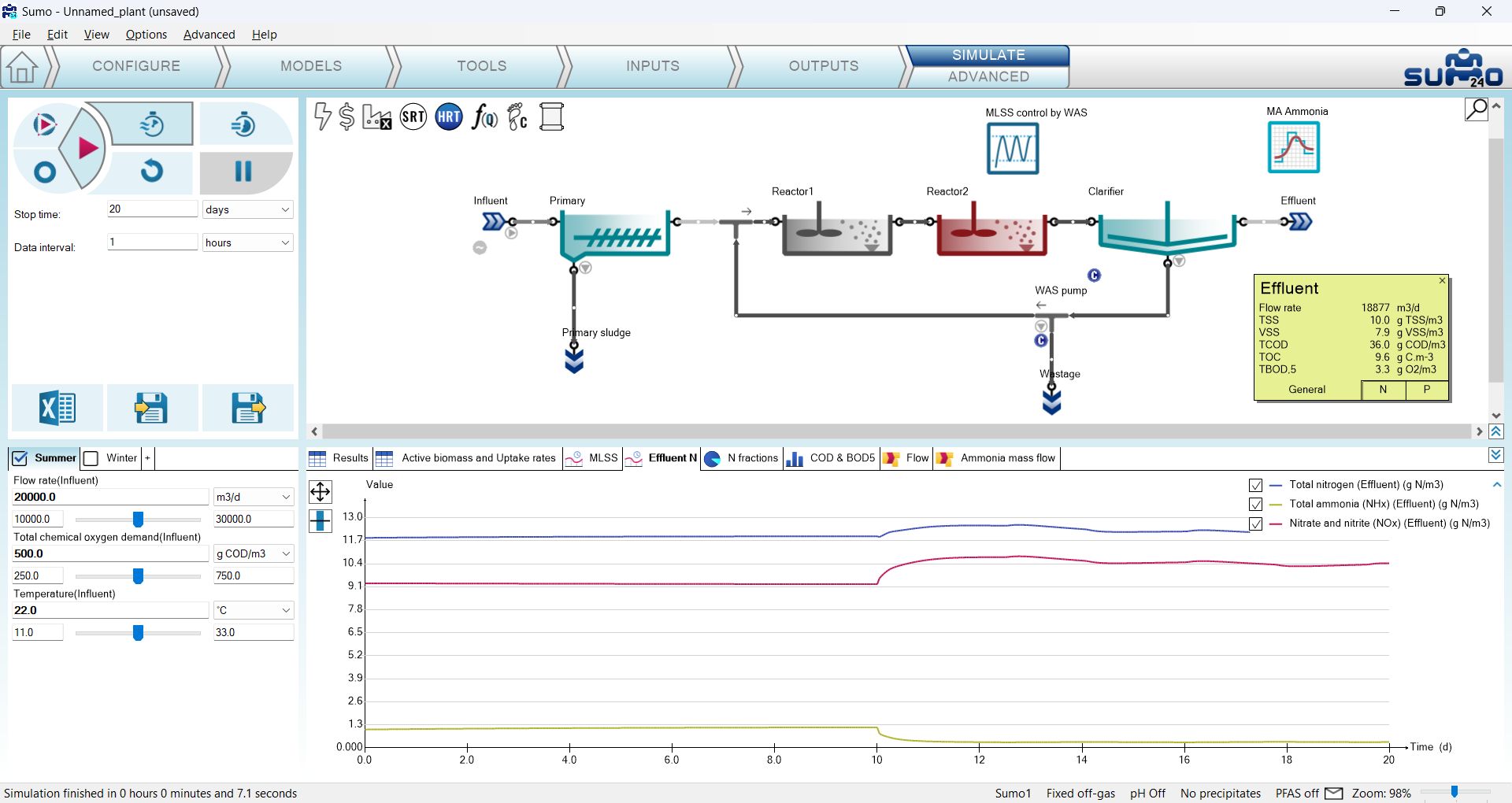
If you hover above any process unit on the Simulate tab with the mouse and leave it there for a second, a yellow popup will appear with a summary table of the most important variables related to that process unit type (Figure 2.7.29). Moving the mouse elsewhere will make the popup disappear soon after. However, if you grab it with the mouse while it is active and place it somewhere in the layout, it will remain there as a sticky note as long as you don't close it with the X in the top right corner. Most popups will have a few tabs in the bottom which you can toggle when the popup is active, in order to reveal more information.
¶ Adding pipe info tables
Data from any table can be set to be shown on the pipes of the layout. For an excercise, let's go back to the Outputs tab and add a table with the Flow rate of the Influent process unit (can be found under Frequently used variables). Rename the table to Pipe info table and right click on the name tab, then click the Show values on pipes option (Figure 2.7.30).
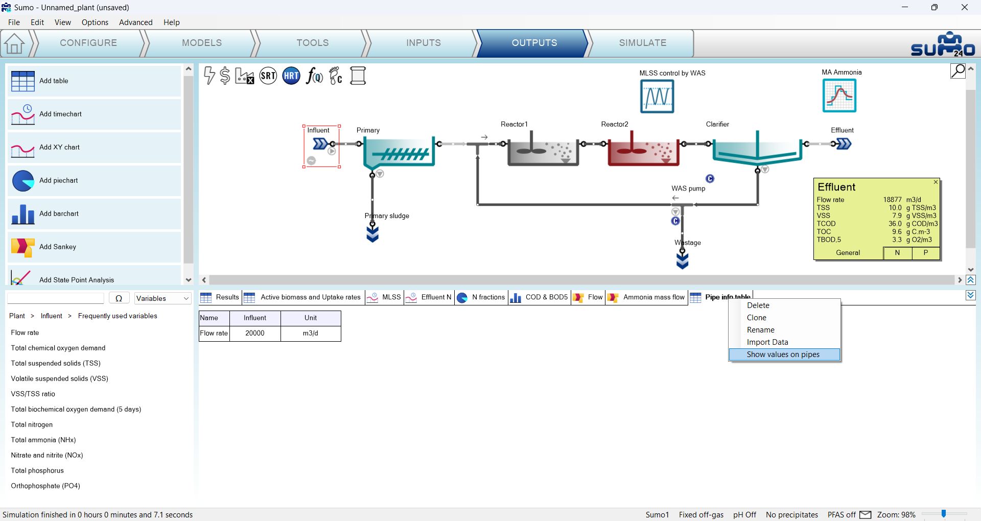
This will add a transparent popup nearby ALL pipes of the configuration. In most cases you will only need a handful of them, so you can remove the unnecessary ones by clicking the X in the top right corner of the unwanted popups. For the exercise, keep only the ones belonging to Influent, Effluent, Primary sludge and Wastage. By dragging and dropping, you can reposition the pipe info popups for better readability. If you add further variables (e.g. to display mass flows or concentrations) to the source table, you will see that they will be shown on the popups as well (Figure 2.7.31). Along the same line, removing variables from the source table will remove them from the pipe info, too.
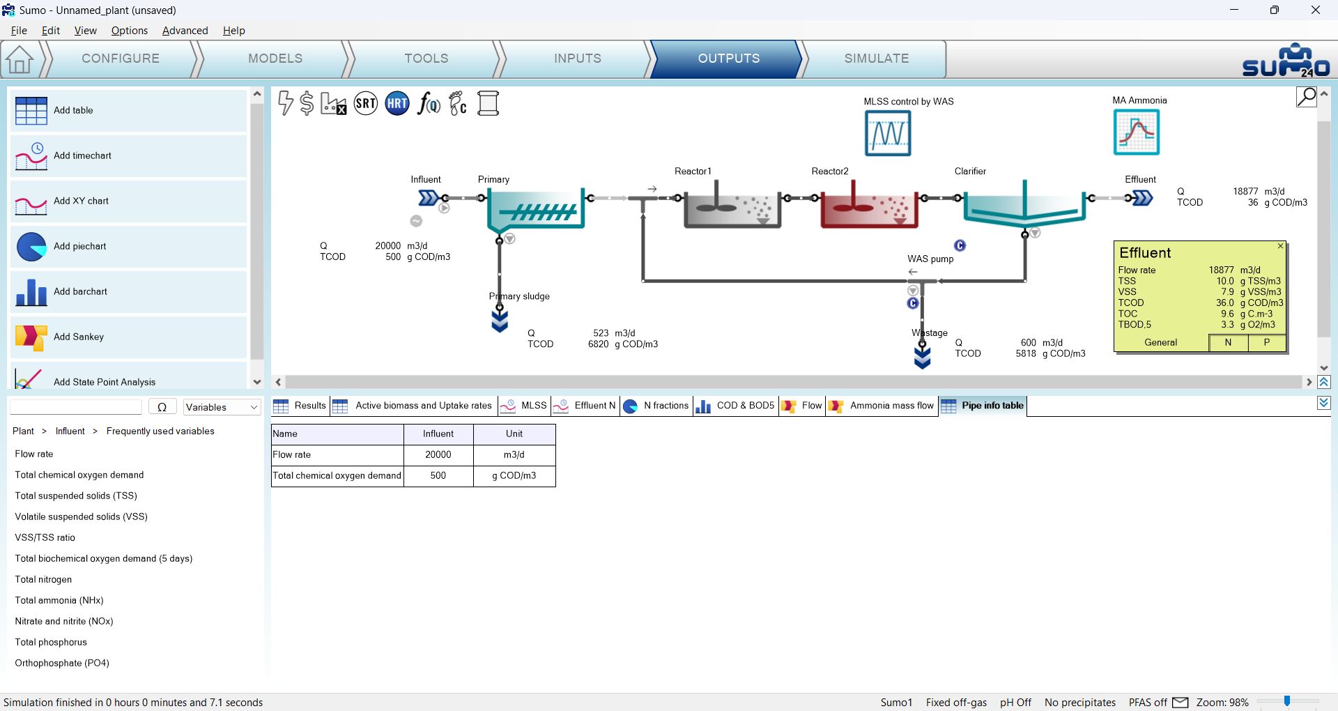
If you wish to switch displaying another table's data on pipes, just simply go back to the Outputs tab, right click on the name tab of the desired table and click the Show values on pipes option there. The content of the pipe info popups will be updated accordingly.
¶ Writing a report
On the Control panel of the Simulate tab, a Report button (resembling a spreadsheet) is available. When clicked (Figure 2.7.32), results will be written to an Excel file (inheriting the name of the SUMO project file by default, but this can be changed), available for further processing. This function creates an Excel file with the following sheets:
- Project overview: contains the configuration layout and basic project information with model (in this example: Sumo1) settings and scenario information
- Notes: the contents of the Notes screen panel from the Configuration tab
- Modified parameters: values of all parameters in the project that were changed from default (including those of controllers and other plantwide calculations like Energy center, Cost center, SRT, HRT, Flow dependence and Plantwide Excel, if used)
- Simulation results: all results of the output tabs get saved to separate sheets, including data tables for the diagrams.
¶ Next chapters
Chapter 3 – Advanced simulations
Chapter 4 – Controllers
Chapter 5 – Energy and Cost calculations
Chapter 6 – Carbon footprint assessment
Chapter 7 – Design model
Chapter 8 – Examples