¶ Introduction
Sumo comes with a set of Excel-based tools to assist your work. This page contains more in-depth information about the available tools in Sumo. We are continuously working on this content to have all the details you are looking for.
¶ How to work with Sumo Excel Tools
In general, Sumo tools are accessible via buttons on the Inputs tab of the relevant process units (e.g. the Influent tool can be opened from the Influent process unit). When you start up a tool from a Sumo project, an Excel file will be opened with the default values. This file will have a unique filename, so that Sumo can assign it to the actual unit and store it within the sumo project file (.sumo, .msumo, etc.) for later use, when it is saved. Thus, multiple Excel tool files can be stored with the project (imagine having multiple influents, each with their own setup, based on data in individual Influent Tool files). This way you can keep all project-related changes to the Excel Tool file(s) within the Sumo project, which comes handy for archiving purposes, as well as when you are working in a group.
If you modify the contents of an Excel Tool file (which is very likely to happen), please make sure that you save it in Excel before saving your project in Sumo, as a project save command in Sumo will pack the saved version of any Excel Tool file that has been associated with the project. So the correct way to handle the management of project-assigned Excel Tool files, is to 1) always save all changes while the tool files are open in Excel and then 2) save your Sumo project.
When a process unit has a saved version of an Excel Tool file in a project, it is indicated by the blue color of the tool button (otherwise being white). If the project is opened again, by clicking the blue tool button on the Input tab, it will open up the relevant file with the last saved data in it.
¶ Influent tool
The purpose of this tool is to help users fractionate their measured influent data into different COD, TKN, and TP fractions that is needed to properly set up the influent model input. Each of the Sumo full plant and focus models have a raw influent and a primary effluent tool which can be accessed by clicking on the influent unit in the Input tab (it is available at the bottom of the screen). The tool is Excel based and is specific to the project and the influent unit. Once the fractionation has been performed, the values should be saved in Excel and become part of the project. This tool will allow users to identify fractions for a constant dataset, meaning, it should be used for average values of a dataset. If multiple datasets are to be fractionated such as winter versus summer, then two tools must be used and saved with different names as part of the project. If the file name is changed, the file can be retrieved from the project directory.
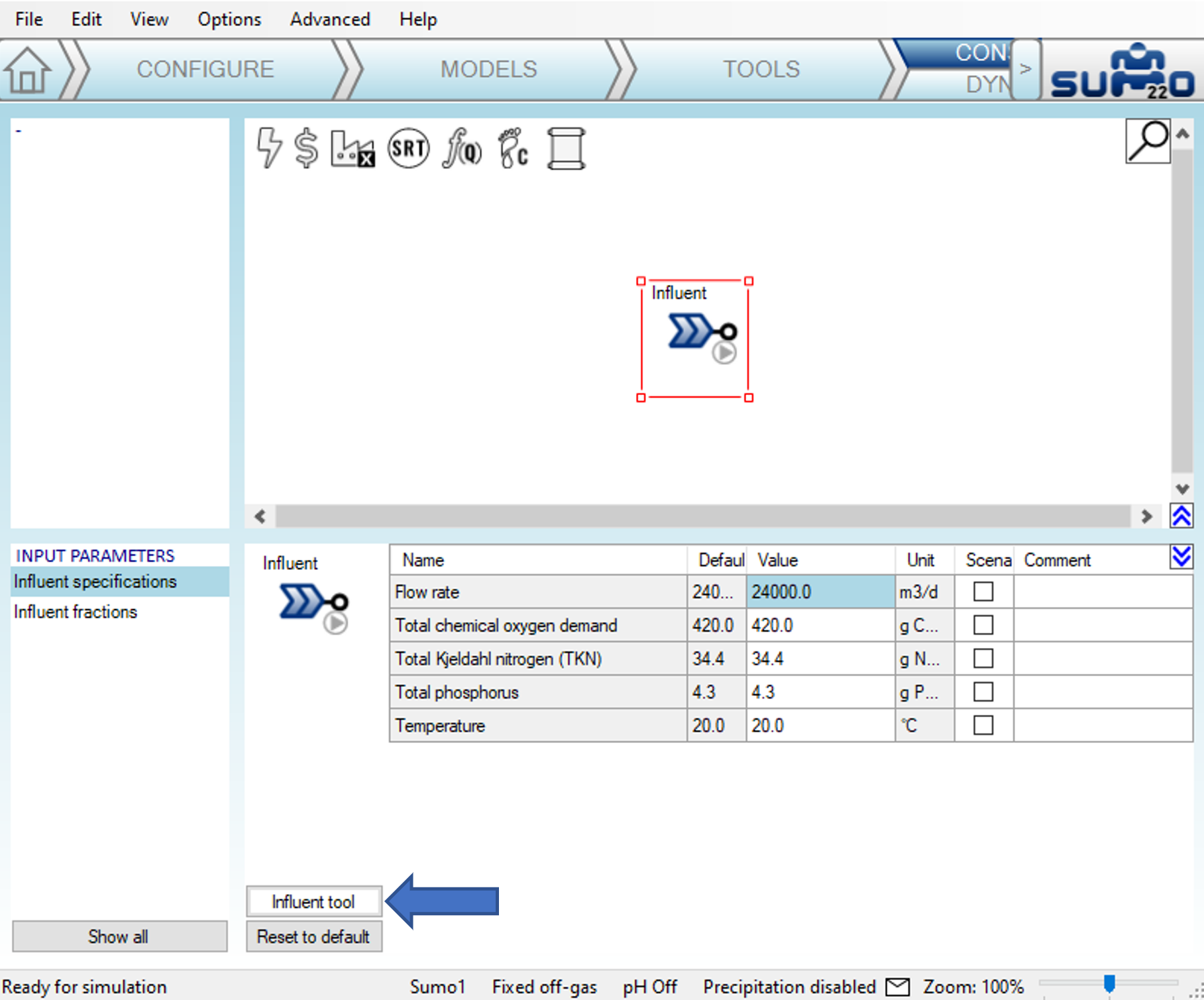
Influent fractionation is one of the key tasks in process modeling and it is very important for users to familiarize themselves with the fractions and the fractionation workflow process. More details can be found in the Influent characterization chapter. Here we present a brief overview of the workflow a user must follow to achieve a successful fractionation and the logic behind the fractionation tool.
¶ Step 1 - Help sheet
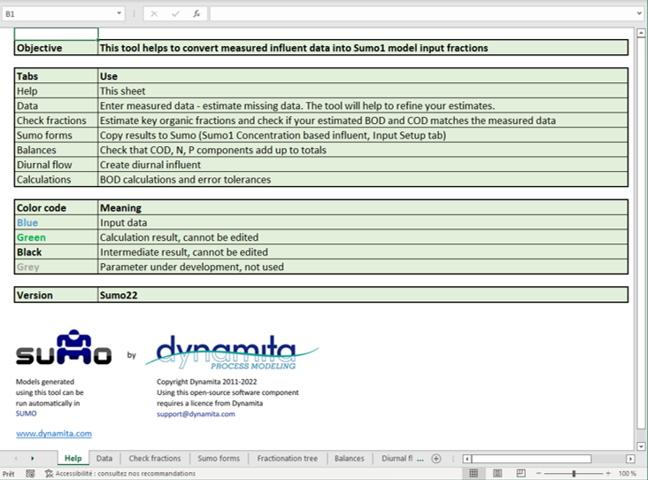
Read the Help sheet, it provides brief information regarding the use of the tool.
¶ Step 2 - Data sheet
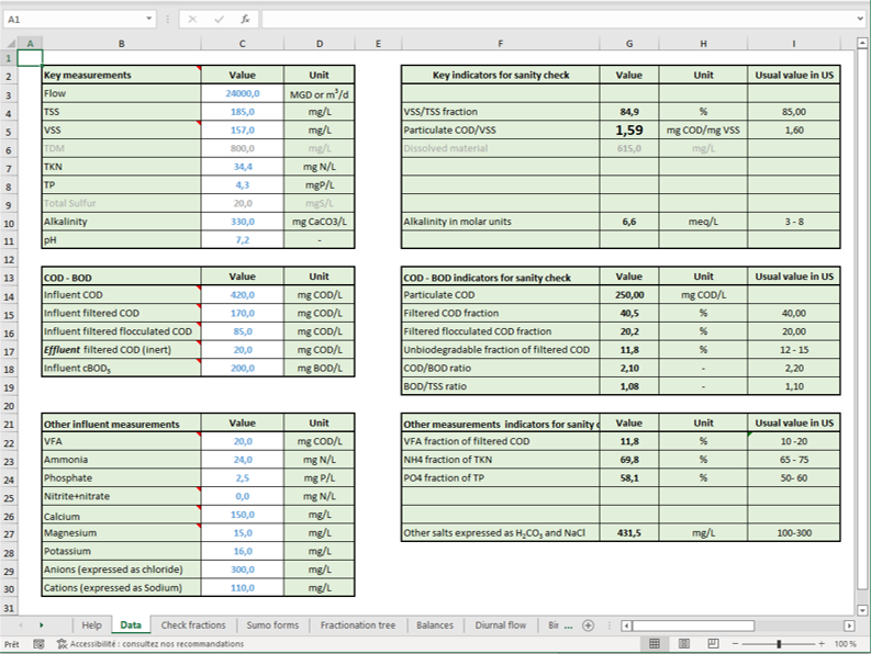
In the Data sheet tool input the available dataset wherever the values are blue (Column C).
- If any of the values are missing, then use the key indicators for sanity check as a guide to estimate the missing values. For instance, if the total COD value is not available then use a typical COD/BOD ratio of your plant or use our recommended value of 2.2-2.5.
- Once all values are provided, the tool calculates key indicators for a sanity check in Column H. One must make sure that they seem reasonable before proceeding.
¶ Step 3 - Check fractions sheet
The Check fractions sheet is for:
- Comparing three main parameters (Calculated influent BOD5, TSS, and VSS) that are provided by the user and calculated based on the fractions identified in Column D of table named Influent fractions to estimate. These fractions can be adjusted to improve the match between data and calculated parameters indicated in COD/BOD/TSS/VSS match table on the right. If comparison is off for BOD by 25% and TSS&VSS by 15% then the verdict will be a no match. Details of the decision matrix can be seen in the Error tolerances table on sheet named Calculations.
The values in the Table called Particulate COD/VSS ratios by component and BOD calculation are used for estimating the parameters as well. These should be adjusted based understanding the type of wastewater user is dealing with.
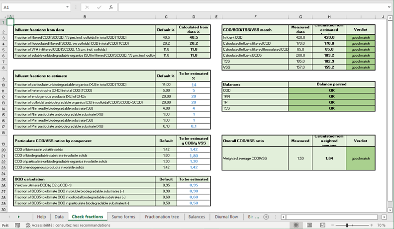
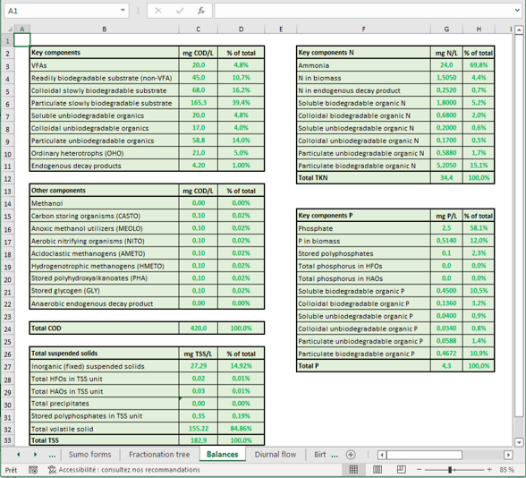
- Checking for the Balances of COD, TKN, TP, and TSS. All the balances must be OK before proceeding. The balance can be off if data or the fractions do not make sense, for instance in the following example: if TCOD is 420 g COD/m3, TKN is 20 g N/m3, and SNHx is 15 g N/m3, there is too little N left for organic nitrogen, and the Tool will tell us that No, please check the data (TKN, Ammonia) and the fractions in the Balances sheet. The details regarding by how much the balance is off can be reviewed in the sheet named Balances. In this case, Particulate biodegradable organic N is -0.1950, which would be incorrect. This can be remedied by either decreasing the fraction of N in readily biodegradable substrate (SB) and fraction of N in particulate unbiodegradable substrate (XU), decreasing the N content of other organics (see table Model parameters in sheet Balances) or the data should be checked for measurement errors.
¶ Step 4 - Feed the parameters to Sumo
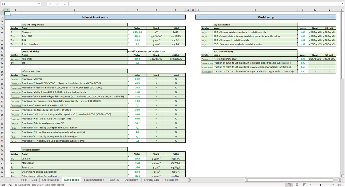
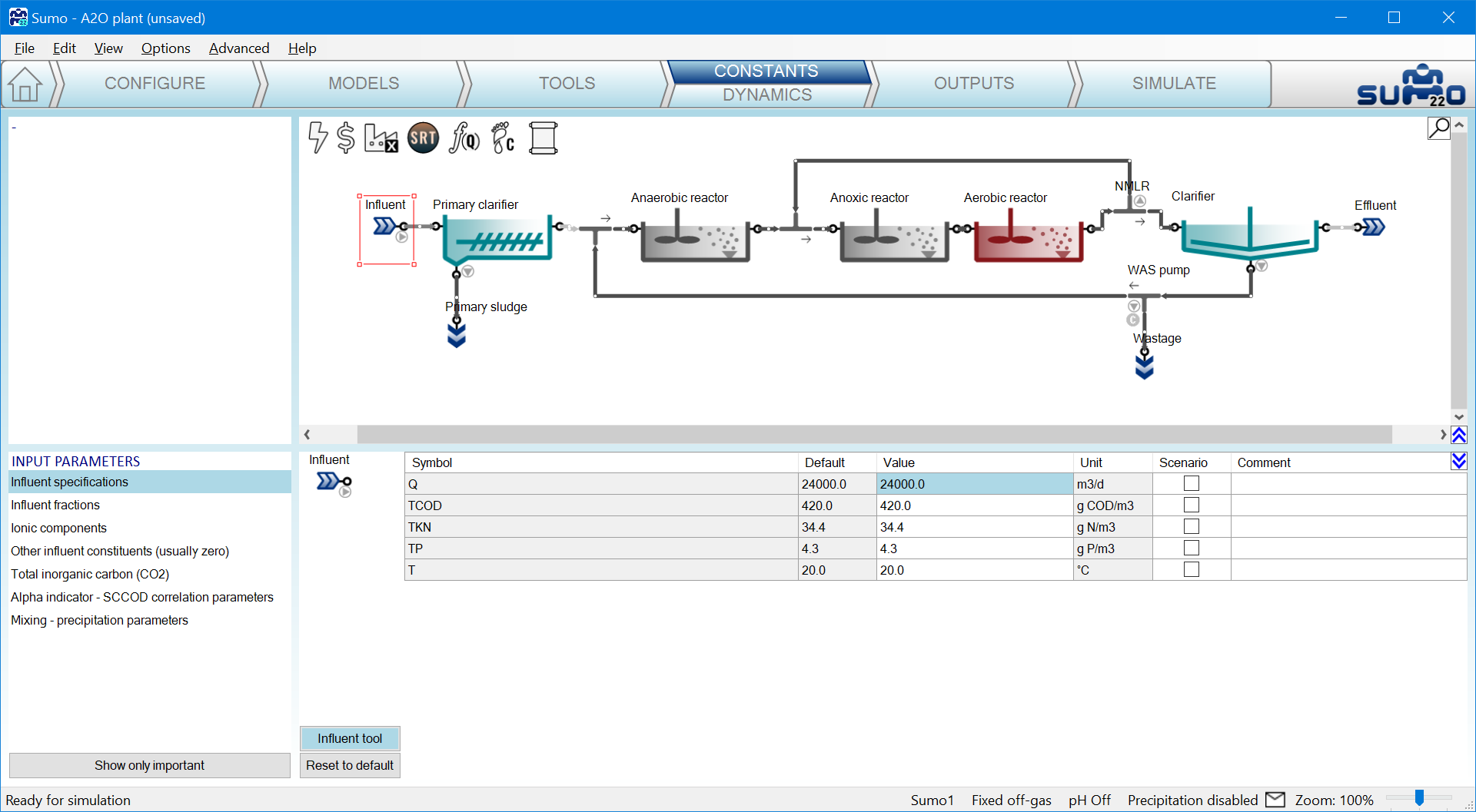
Copying the values from the tool’s Sumo form to the Sumo influent unit can be done by selecting, copying (Ctrl-C), and pasting (Ctrl-V) in Sumo.
|
|
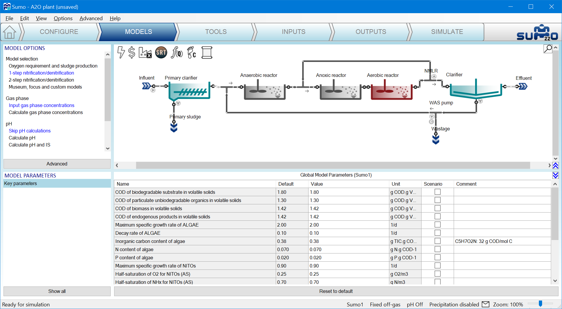
If any of the model parameters including COD/VSS ratios were adjusted, then they should be copied to the Model Setup tab in Sumo.

|
|
Note: in some cases the computer struggles to get the information from the clipboard in a few milliseconds. In case of struggling to paste the information, hold the Ctrl-V a bit longer once the first cell of paste is selected (select only, do not go to edit the cell mode).
¶ Other features of the tool
¶ Fractionation tree
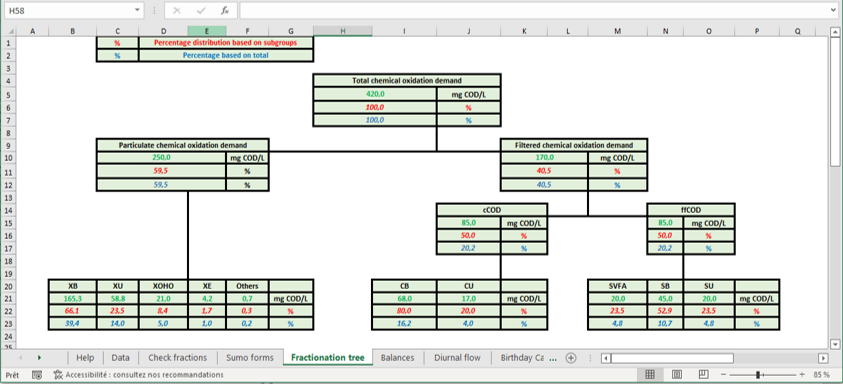
The fractionation tree sheet helps you visualize fractions and are useful for documentation.
¶ Diurnal flow
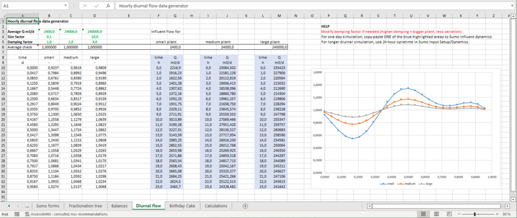
The Diurnal flow sheet creates three types of hourly dynamic influent data (small, medium and large plants) for 24 hours using the Flow value provided in the C3 of Data sheet. This dynamic table is useful for setting up dynamic simulation in case no diurnal data is available.
Birthday cake
The Birthday cake sheet provides hourly data for a simplified birthday cake analysis of 16 days. This is useful for sizing and evaluating plant performance under diurnal variation, monthly maximum load and peak daily load conditions. For further details we suggest to look into the Guidelines for Using Activated Sludge Models published by IWA.
¶ Note
There are multiple situations all of which can not be described comprehensively in this document, so refer to the Influent characterization chapter and feel free to write to support@dynamita.com.
¶ Aeration (SOTE) tool
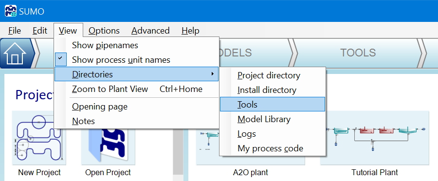
The purpose of this tool is to identify parameters for the clean water oxygen transfer modeling function through curve fitting using diffuser equipment testing data. The tool can be reached from View|Directories|Tools folder by opening Dynamita aeration (SOTE) tool.xlsm.
Be aware that the tool is using VBA macros that require certain Microsoft libraries to be activated in order to run. Should you experience compile errors while using some of the tool's functionalities, please open Visual Basic from the Developer menu (you can show the tab from the Customize the Ribbon…menu item), then select References from the Tools menu, and ensure you have enabled the following references:
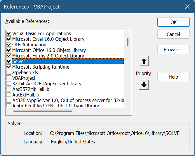
To ensure that the Solver add-in is available in Excel please click File > Options > Add-ins > select “Disabled add-ins” from the list > Go > Enable Solver, then you can access File > Options > Add-ins > Select "Excel add-ins" > Select "Solver" from the list.
You can save the tool anywhere, even drag and drop the file to the Notes (bottom right panel) on the Configure tab in Sumo so it will be stored with your project.
¶ Step 1 - input parameter set definition
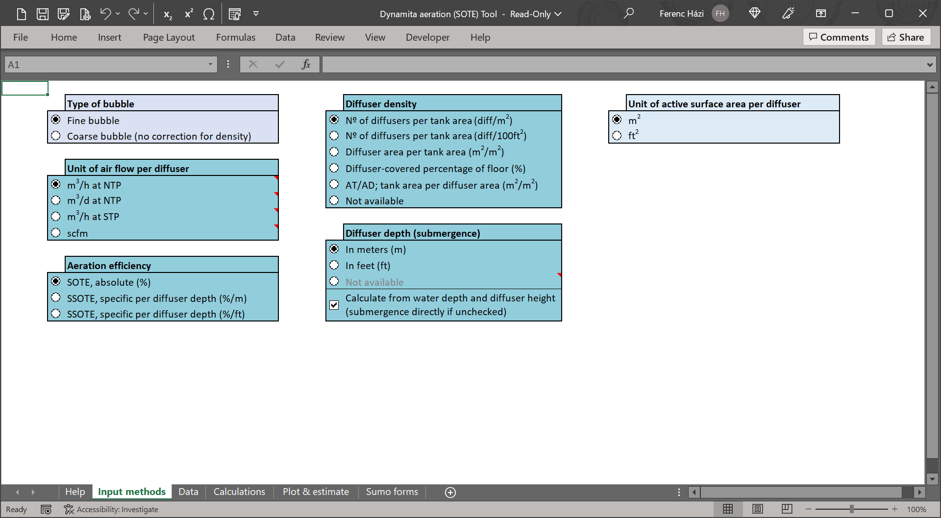
The parameters identified are plugged into the Oxygen transfer efficiency correlation parameters table in the reactor model for calibration of the plant’s diffuser system. In the Input methods sheet, users start by selecting the type of diffuser and the units for key information to be processed by the tool. The selection criteria are presented below.
¶ Step 2 - Provide data
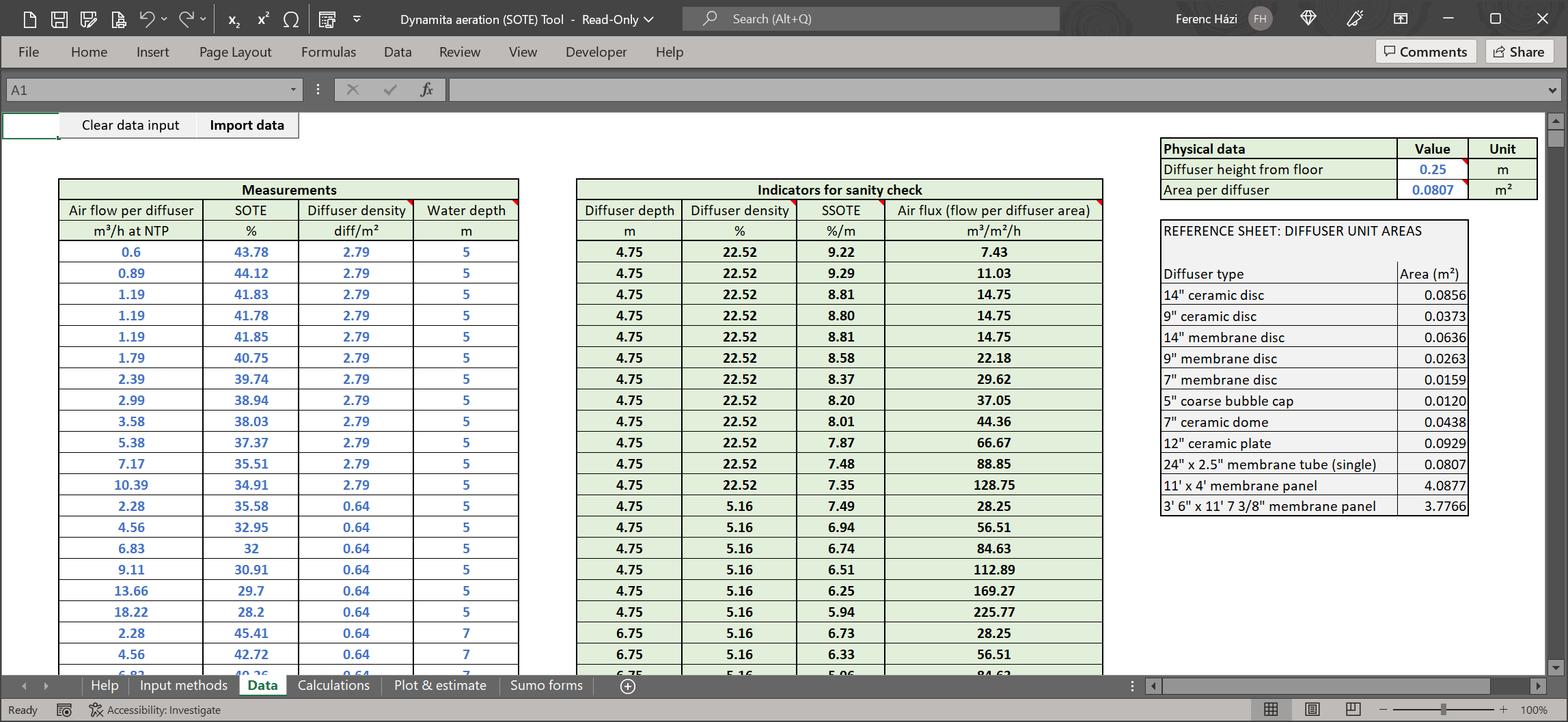
Next step is to switch to the Data sheet and provide data from manufacturer specifications or plant measurement campaigns within the Measurements table and provide the Physical data such as Diffuser height from floor and Area per diffuser. The tool comes with a default set of demonstratory data which must be removed by clicking the Clear data input button at the upper left corner of the sheet. Also available is a reference sheet containing common diffuser type unit areas, for estimating the active surface area. Once the new data is entered, users must press the Import data button to start the automated data manipulation. The details of these calculations can be seen in the Calculations sheet where the dataset is processed for curve fitting.
¶ Step 3 - Check parameter fitting
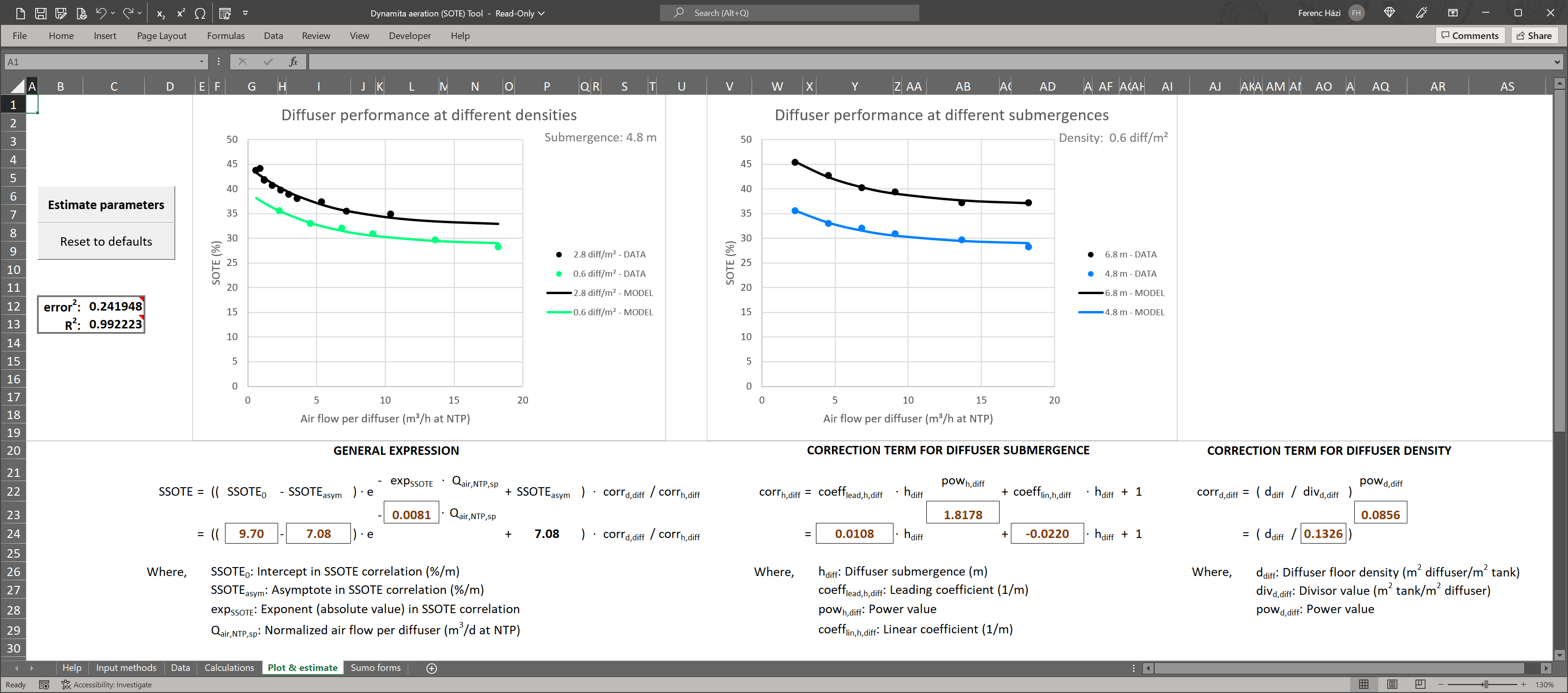
In the Plot & estimate sheet the parameters are estimated for the expression predicting SSOTE, including the correction term for diffuser submergence and the diffuser density by adjusting the function parameters to match the measured data (Estimate parameters button on the left side of the sheet). See the figure below showing the fitted curve.
¶ Step 4 - Feed the parameters to Sumo
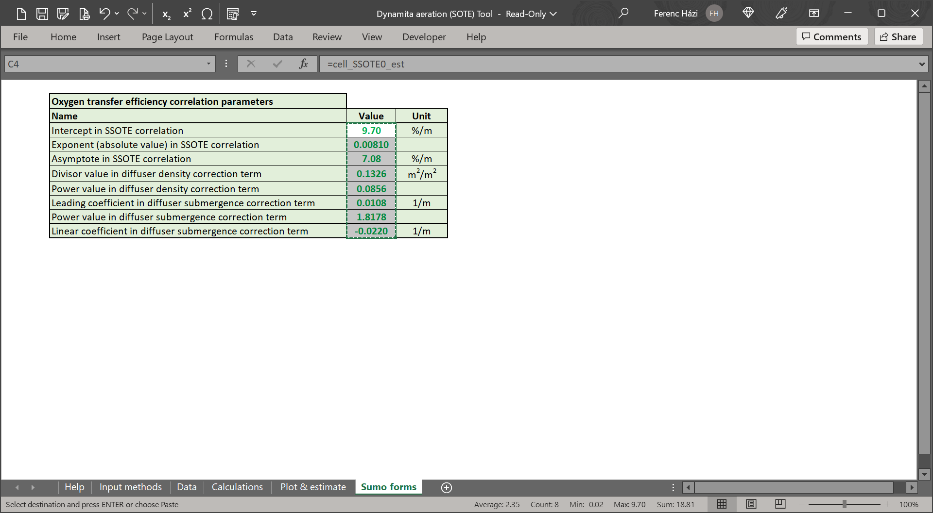
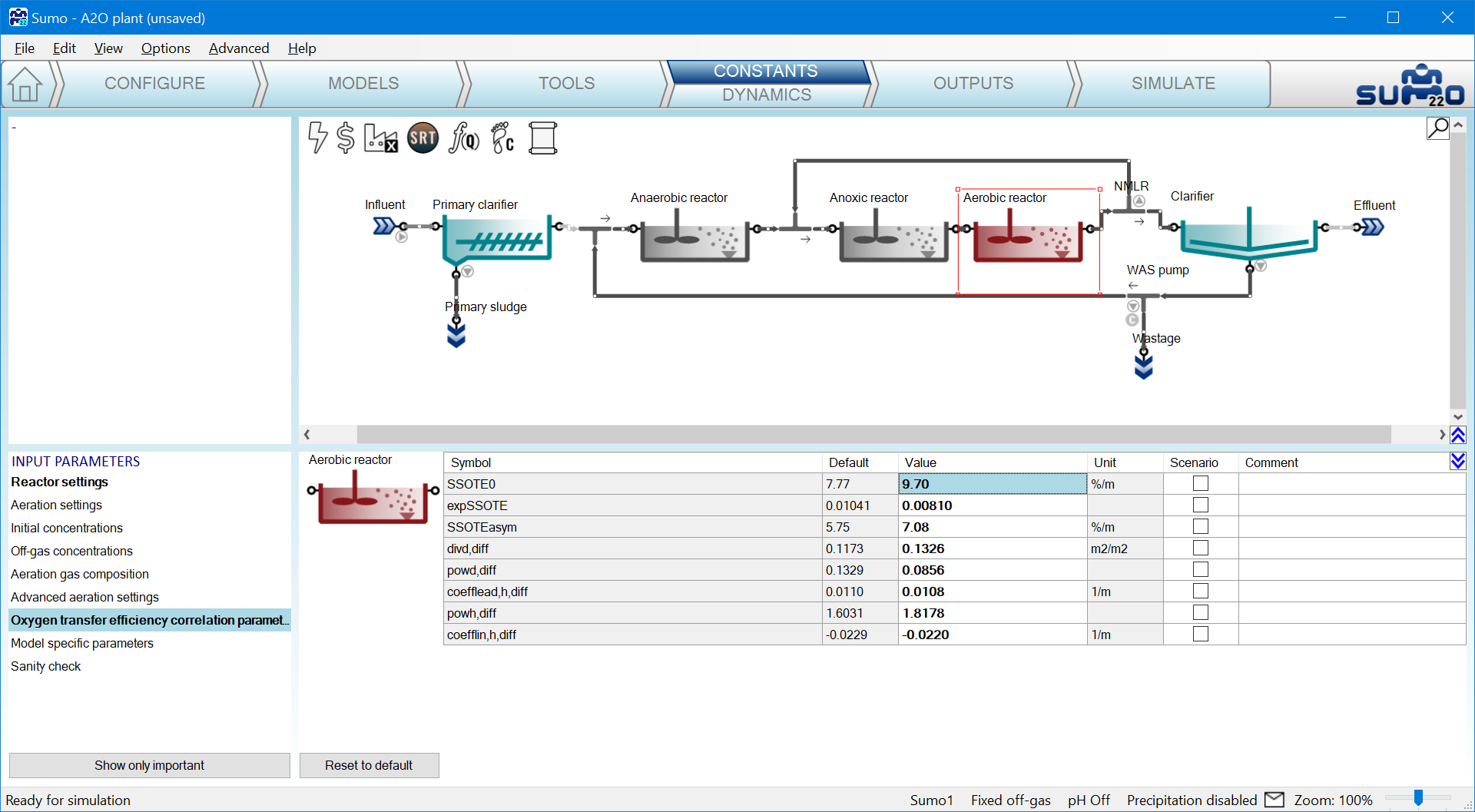
The last step is to copy the values from the Sumo forms sheet in the tool into the reactor’s Oxygen transfer efficiency correlation parameters in Sumo within the Inputs tab.
|
|