Dynamita, www.dynamita.com, Sigale, France
Sumo is a third generation wastewater process simulation software. It was put together by a dedicated team with professionalism and thousands of days of tender loving care. Enjoy, and please let us know if you find somewhere it is coming short of your expectations. We will do our best to improve it.
Imre Takács, on behalf of the whole Dynamita team
Sigale-Toulouse-Budapest-Toronto-Innsbruck
Released: September, 2022
Last updated: April, 2024
¶ Contact
This Manual, the Sumo software, SumoSlang and related technologies are the copyright of Dynamita.
Copyright 2010-2024, Dynamita
Dynamita SARL
2015 route d’Aiglun
Sigale, 06910
France
Mobile in France: +33.6.42.82.76.81
¶ Installing Sumo
The following steps will help to guide you through the installation of Sumo.
¶ Prepare Microsoft Windows for Sumo
Operating system
Make sure your computer is operating Microsoft Windows 7 or later. Sumo supports touch screen computers running Windows 8/8.1 and Windows 10/11.
Sumo can be used on a Mac with Windows installed or through an emulator like “Parallels”.
Microsoft Office
Sumo requires Microsoft Excel 2007 or later installed.
.NET
Please make sure that your computer is running the Microsoft .NET 4.7.2 framework. You can check it in the list of installed applications (Control Panel / Programs / Programs and Features). If the .NET framework’s 4.7.2 version is not installed, please download and install it from the following location:
https://dotnet.microsoft.com/download/dotnet-framework/net472
Windows 10/11 come with the required .NET environment. On other operating systems, if you have .NET already installed on your computer, the downloaded installer will exit or inform you. Proceed to the next step.
¶ Installation of Sumo
You have received a link to the Sumo installer (or in rare cases the install file on a USB key). This is one file and contains everything necessary to install Sumo once Windows is prepared. Download it through the link provided to your computer. From the USB key you can install directly if desired, it is not required to copy the file to the computer.
Install Sumo by starting the install package and follow the instructions. Administrator rights may be required during installation. For workstations, we recommend choosing the “Install for myself only” option.
¶ Obtaining a license
Obtaining a license is a two-step process.
¶ Step 1:
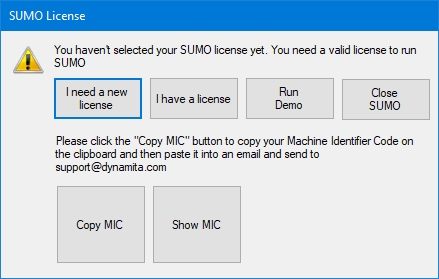
After install, start Sumo from the Windows Start menu. Sumo will display a message providing multiple options. If you don’t have the license file yet, Select “I need a new license” (Figure 1.1). Sumo will display two additional buttons to show information about your hardware (Machine Identifier Code) and to copy this information directly to the Windows clipboard. Please paste this code into an email and send it to support@dynamita.com. Dynamita will provide a license file for you according to our agreement.
¶ Step 2:
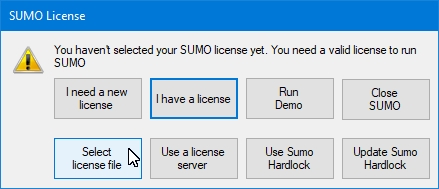
Copy the license file Dynamita provided to a folder on your computer, start Sumo, choose the “I have a license” option, click “Select license file” and navigate to load the license file (Figure 1.2). As long as the license file is not deleted or moved and it is valid, this validation does not have to be repeated. Other options, like using a license server or a hardlock, are also available.
¶ Note: Demo license
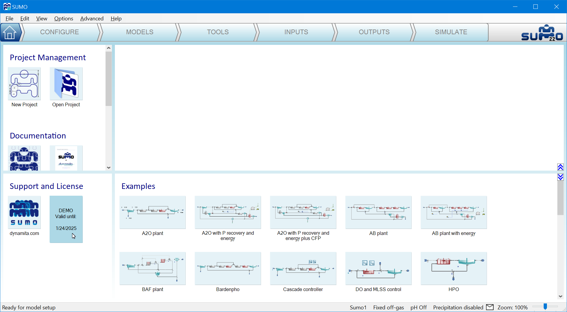
If you already have Sumo installed and running in demo mode, you can go to Step 1 by choosing the “Home” icon and selecting the licensing button in the bottom left window pane.
¶ Introduction
Sumo is a powerful, open process source, multipurpose simulation environment developed for environmental models, particularly municipal and industrial wastewater treatment plant modelling. A wide range of BNR plant configurations can be simulated in Sumo. Sumo models are written in an Excel based open process source code language called SumoSlang (Sumo Simulation Language, copyright Dynamita).
Sumo can simulate traditional biokinetic models dynamically or in steady-state, mixed equilibrium-kinetic models and direct algebraic models, depending on the simulation mode.
Sumo is supplied with internally researched and developed whole plant models as well as focus models (e.g. with focus on sulfur, high rate plants and the fate of nitrogen and GHG). The seven most widely known published models are also included in the Sumo Museum for N and P removal.
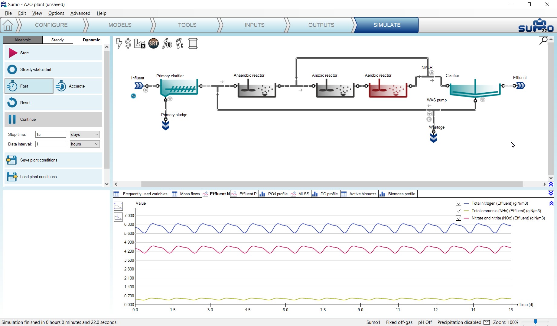
Sumo models can be run through several different interfaces. The most widely used is “Sumo”, an intuitive graphical user interface (Figure 2.1).
Sumo22 is able to communicate with other programs such as Excel, Python, Matlab, etc., through its Digital Twin Toolkit (DTT). The Sumo22 install comes equipped with a couple of examples:
- Excel based “Operator interface”. This can be customized to a certain plant configuration or SCADA for easy use of plant simulations.
- Sample Python scripts for sensitivity analysis and parameter optimization using Sumo.
Please note that the Digital Twin Toolkit (DTT) will only work with a valid DTT license, which is available separately from the Sumo license.
¶ How to use Sumo for simulations
¶ Start Sumo
On Windows 10 systems, you can use the start menu to launch Sumo. The installer places the software in a folder called “Dynamita”. A quick way of locating the application is to start typing ‘sumo’ once the start screen is on (Windows 10 switches into application search mode in this case, showing the most relevant search results on the left). With drag and drop, you can also pin a Sumo22 quick launch icon to the Start menu tiles or to the Desktop of the computer as well. Note: right clicking on the program launcher icon allows you to open the recent project files.
Sumo will start with showing the Welcome Screen, as illustrated by Figure 3.1. Below the Menu Bar, you will see the Task Bar that guides you through the project workflow, all the way from configuration to simulation.
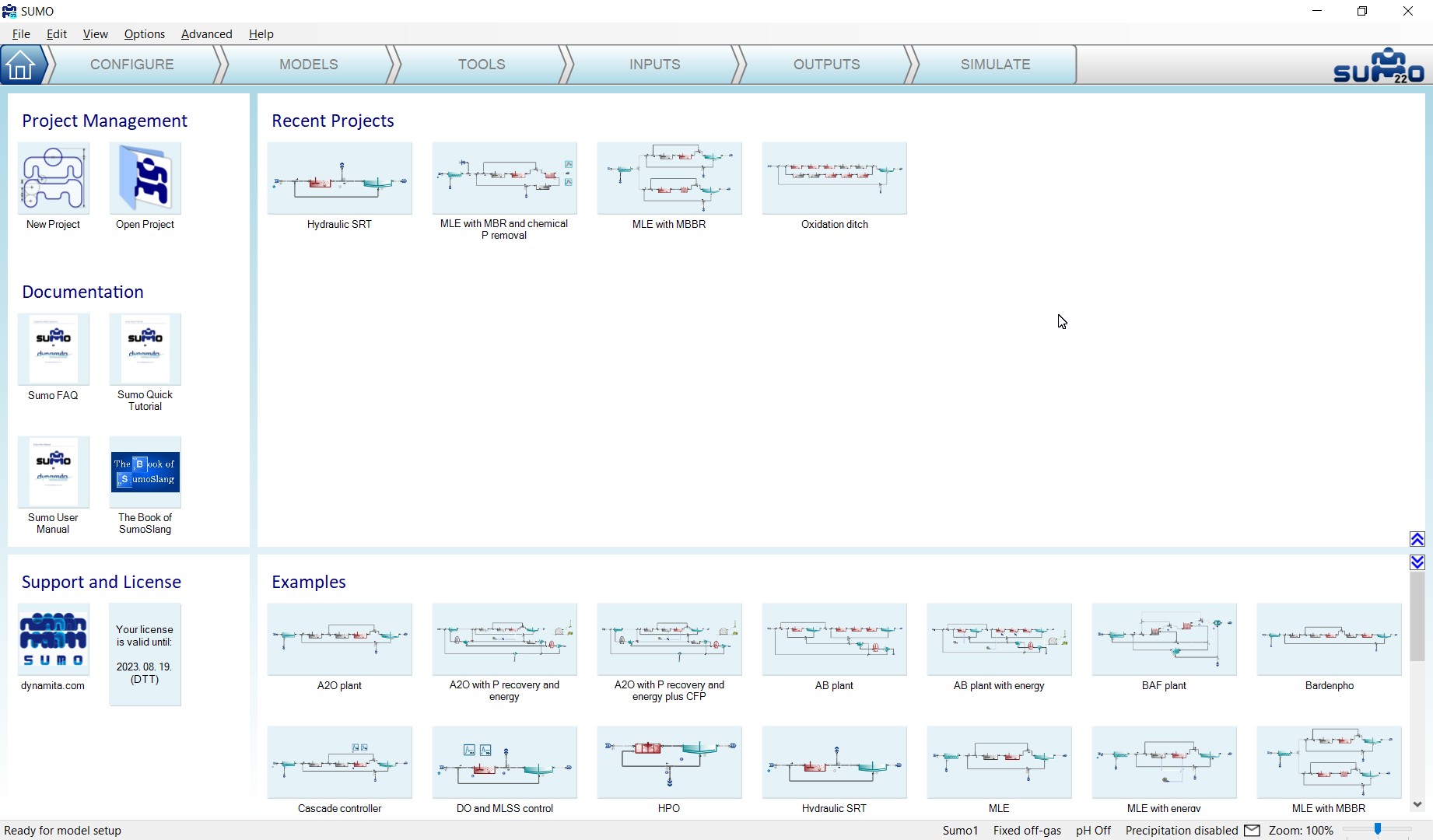
The central elements of the Sumo22 Welcome Screen are four screen panels, whose functions and roles are the following:
| Top left panel |
Project management and documentation Starting or opening a new project in a new window (New Project), opening a saved project from your own files (Open Project) and reaching various documents for how-to-use instructions. |
| Top right panel |
Recent projects Your recently opened projects can be quickly reached from the welcome screen. |
| Bottom left panel |
Support and license information Sumo22 support (link to our website) and the currently used license information can be reached from here. |
| Bottom right panel |
Built-in example project repository All the built-in example configurations can be opened directly from this pane (they are also available from the Help menu). |
These functions can be reached later at any point, by clicking either the Home icon (the first item of the Task Bar) or the Sumo22 logo (located at the right end of the Task Bar), which will bring you back to the Welcome Screen.
The screen panels can be resized anytime during the workflow to fit the actual needs of the job. In order to do that, just move the mouse to the padding between the panels and drag them to the desired position. The top right panel will always contain the plant configuration, while the content of the other panels depends on the actual task (Configure, Modes, Tools, Inputs, Outputs, and Simulate). Please note that the runtime versions of Sumo are not meant for constructing new models and thus, the Configure, Models and Tools tabs are not available.
The Status Bar in the bottom of the screen provides model/simulation related information. In case of a system notification or model/simulation error, an exclamation mark will appear next to the mailbox icon (Figure 3.2). Red exclamation marks denote errors, while blue and yellow ones inform about warnings and notifications that need attention. Clicking on the mailbox icon will provide the description of the problem and hints about dealing with it.

The following chapters will help you to understand the functions of each main tab of the Task Bar, and teach how to use them for building a project and performing various simulations.
¶ Configure
To start your project, click on the New Project icon or the Configure tab. This task serves the building of the plant layout.
The roles of screen panels in Configure mode are the following:
| Top right panel | Plant configuration drawing board |
| Top left panel | Process unit categories and process units |
| Bottom right panel | General comment panel – your notes, which will be saved with the project |
| Bottom left panel | Specific process unit options and information |
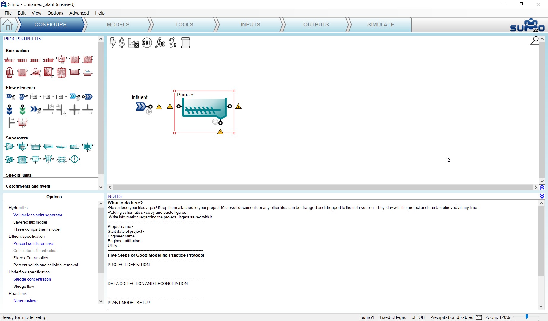
While the Configure tab is selected, we will build a simple AO configuration (also available for reference from the built-in examples as Tutorial plant) using the Flow elements, Bioreactors and Separators categories from the top left element list. Select the desired process unit by opening the category and dragging the process unit to the drawing board. To drop the selected unit, just release the mouse button (Figure 3.3).
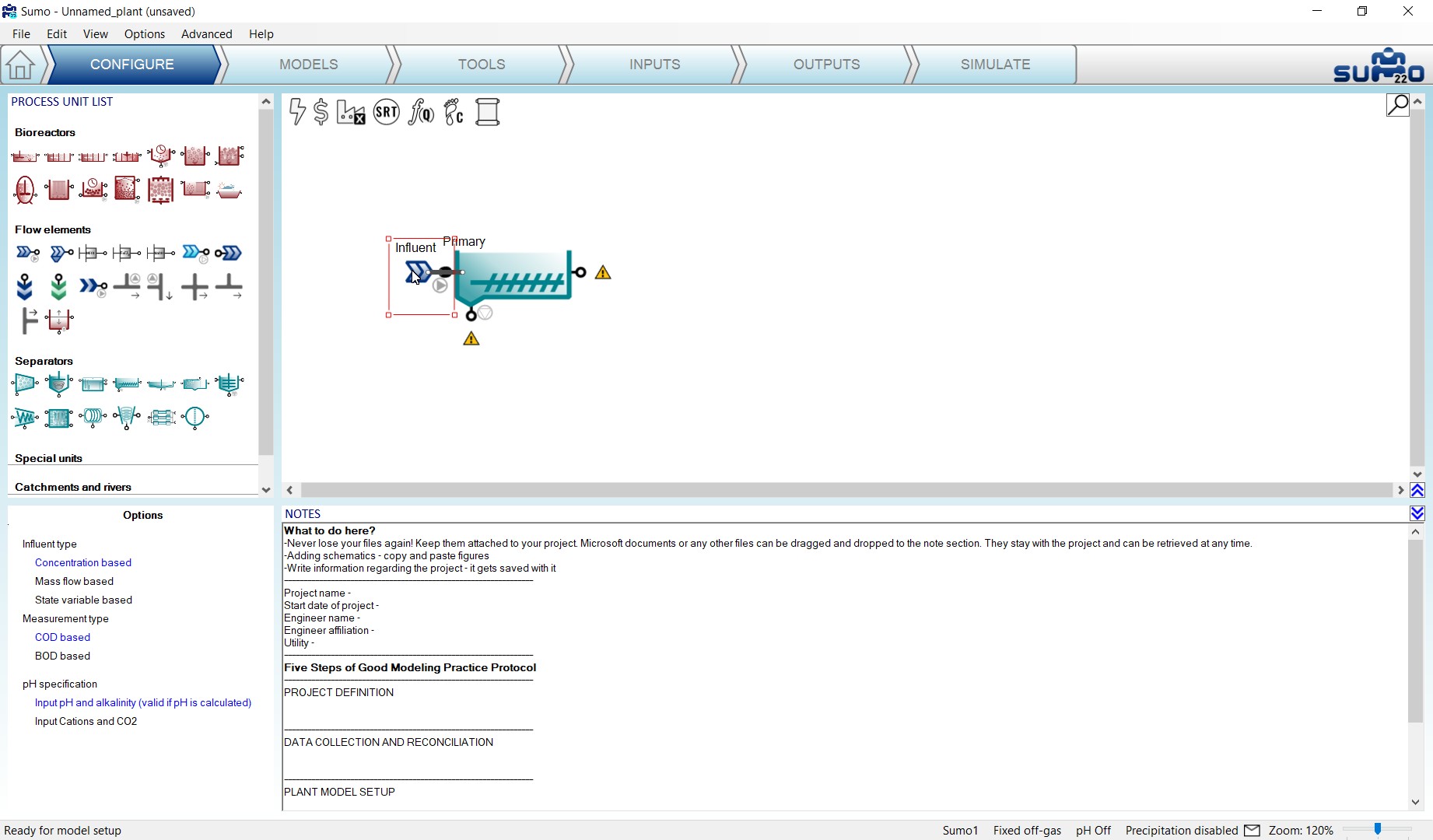
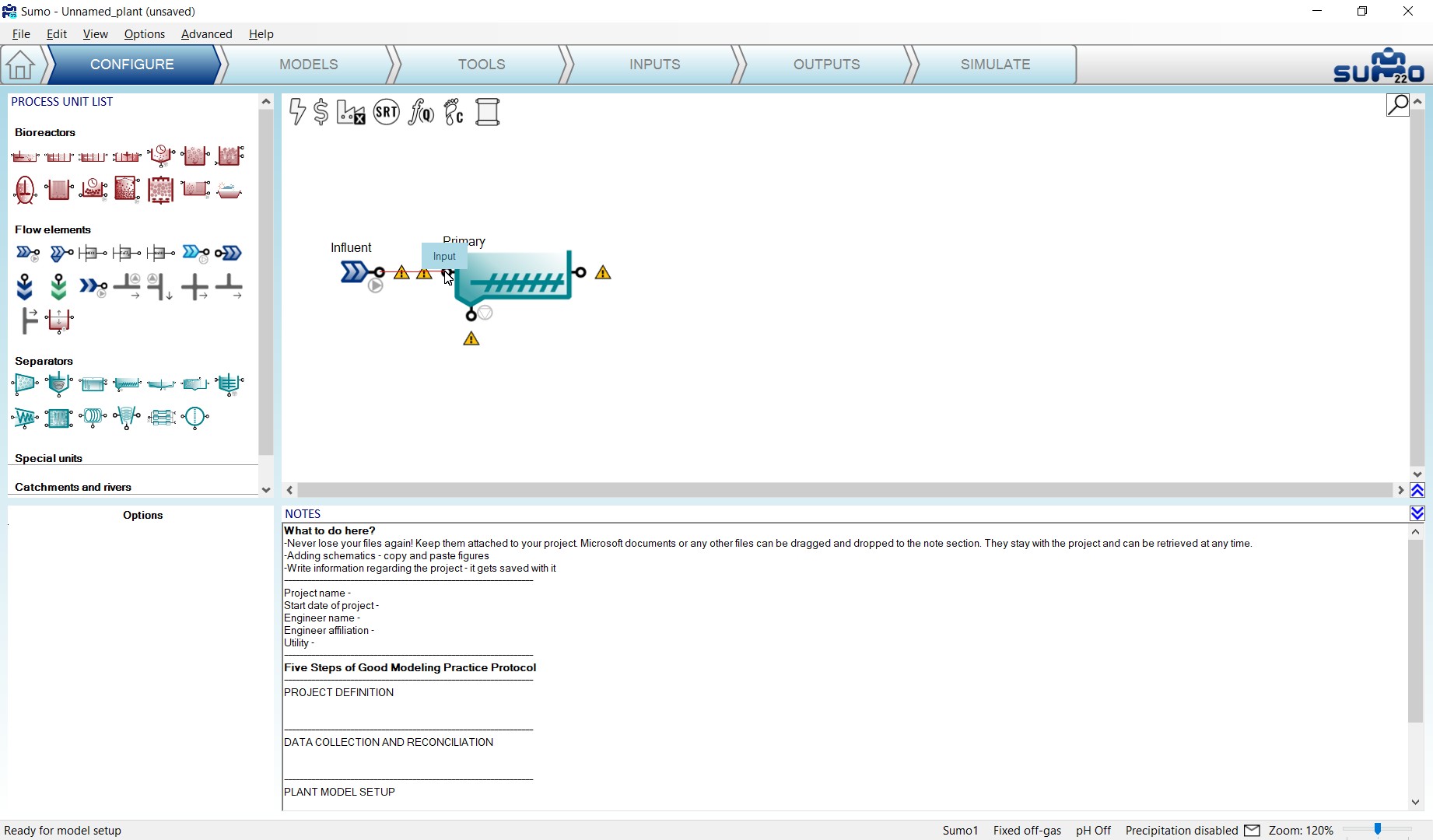
Pipes can be created using two methods. Sumo supports a handy way of establishing connections between process units, which can be triggered by positioning a process unit’s output port on top of another process unit’s input port (or vice versa) by moving one of the process units. Once the ports are positioned on top of each other, a pipe connection is automatically created, as it is demonstrated by Figure 3.4 with an Influent and a Primary clarifier. This method is especially useful when Sumo is commanded by fingers on a touch screen. Unconnected ports are indicated by yellow exclamation marks in the Configure and Models tabs.
The conventional way also works: position the mouse on an output port of a process unit, press the left mouse button, then move the mouse – and this way drag the pipe, denoted by a red line – to an input port of another process unit (as illustrated in Figure 3.5) and finally release the mouse button to make the connection. Existing pipes can be removed by right clicking on them and selecting Disconnect pipe from the pop-up menu.
Build the plant configuration and connect the pipes as shown by Figure 3.6. Tooltips provide hints about the purpose of a unit’s connection point. This feature comes especially handy for the flow divider and flow combiner (make sure not to mix up these connections – their name is shown on a pop-up tooltip and flow direction is indicated by small arrows). Rotate the flow divider below the clarifier by swiveling the red selection rectangle (or with a right click pop-up menu option) and straighten the lines by grabbing process units or pipe corners. These maneuvers do not change the results of the simulation but will make working with the model a lot clearer.
Upon selecting a process unit on the drawing board, options appear in the bottom left panel, where the most suitable process unit can be chosen, fitted to the model. In this Tutorial we will use:
| Influent | |
| Influent type | Concentration based |
| Measurement type | COD based |
| pH specification | Input pH and alkalinity (valid if pH is calculated) |
| Primary | |
| Hydraulics | Volumeless point separator |
| Effluent specification | Percent solids removal |
| Underflow specification | Sludge concentration |
| Reactions | Non-reactive |
| CSTR (both) | |
| Dissolved oxygen | Input |
| Aeration | Diffused |
| Reactions | Reactive |
| Reactor type | Mainstream |
| α factor specification | Predicted α |
| Diffuser system specification | Membrane discs |
| Clarifier | |
| Hydraulics | Volumeless point separator |
| Effluent specification | Fixed effluent solids |
| Underflow specifications | Sludge flow |
| Reactions | Non-Reactive |
| Side flow divider | |
| Flow divider options | Side flow divider with side pump (with cycling turned off) |
Note: The flow divider’s connection where the small pump symbol points to needs to be connected to the waste sludge and the other output (where the arrow points to) will be the recycled activated sludge.
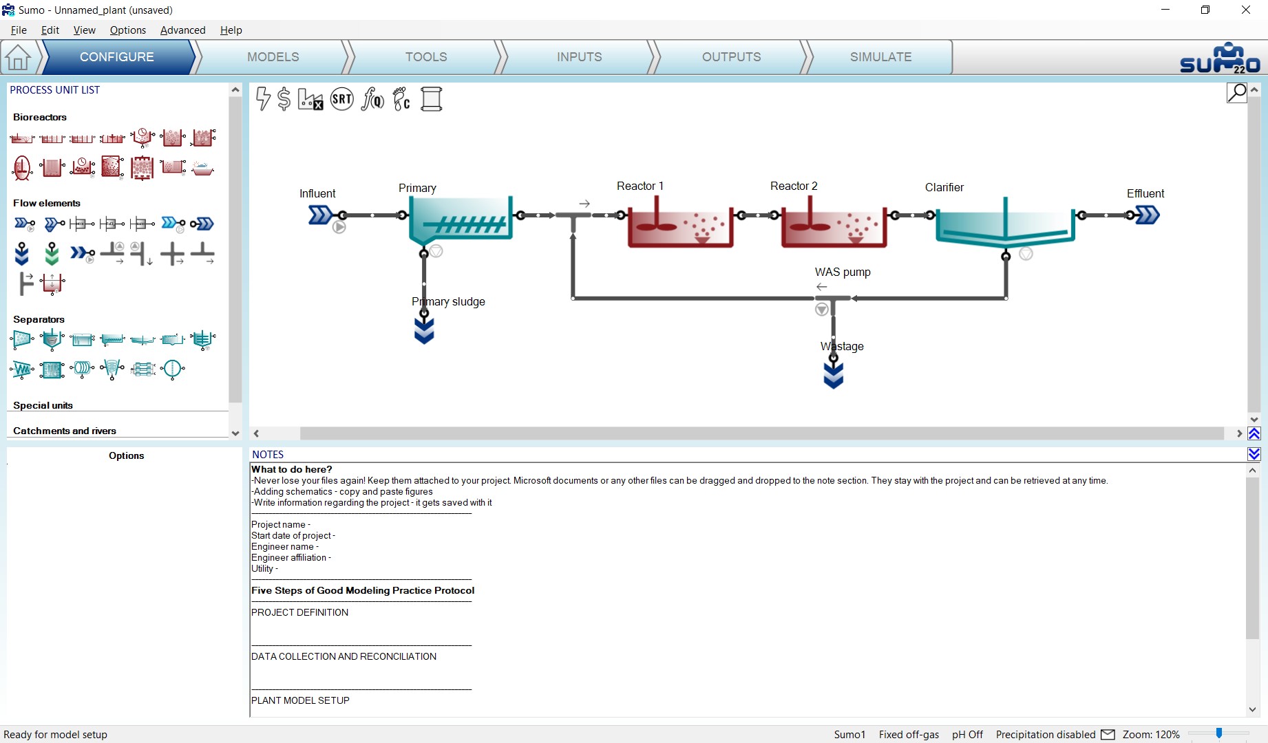
The drawing board can be easily zoomed in and out by holding down the CTRL key while scrolling with the mouse wheel, or alternatively by adjusting the zoom slider in the right end of the Status Bar. To move the configuration around the pane, hold down the CTRL key and the middle mouse button simultaneously while moving the mouse. To fit the actual configuration in the center of the viewport with the optimal zoom level, press CTRL+Home.
Rename the process units using the right-click pop-up menu, the F2 function key or double-click on the upper part of the unit. The pipes can be renamed as well, but this is usually not important – the pipe names are hidden by default (this can be changed in the View menu on the top). The visibility of process unit names can be controlled on a one-by-one basis. In order to obtain a clear example layout, hide the name of the ‘Side flow combiner’ process unit (this is the default setting).
Note: the above settings can only be modified in Configure mode, but you can return and perform them at any point during your work. Changing the process unit names will not result in recompilation of the project model.
Note: other process units (e.g. Sewer network and Mobile carrier) may be available as add-ons. Please write to support@dynamita.com for information.
¶ Models
In this optional task, the mathematical model describing the biological, chemical and physical processes can be selected. If no settings are changed, the default settings will be used – the model will be functional.
The role of screen panels in Models mode are the following:
| Top right panel | Plant configuration |
| Top left panel | Available model options or models in advanced mode |
| Bottom right panel | Model parameters |
| Bottom left panel |
Model parameter categories Note: in the case of Sumo models, only selected key parameters are shown by default; click on the Show all button to see the entire parameter set. |
In this task, we can choose between using the various built-in models for our plant, as well as additional options like turning on or off gas phase, precipitation and different complexity levels of pH calculations.
The current package comes with the Sumo whole plant models listed in Table 3.1.
Table 3.1 – Description of Sumo whole plant models
| General full plant models | |
| Mini_Sumo |
Simplified One step whole-plant model Use “Mini_Sumo” for OUR and sludge production prediction. |
| Sumo1 |
One step whole-plant model Use "Sumo1" for activated sludge modeling, iron addition for P removal and with plants that have digesters but no iron addition. |
| Sumo2 |
Two step whole-plant model Use "Sumo2" for activated sludge modeling and sidestreams, iron addition for P removal and with plants that have digesters but no iron addition. |
| Focus models | |
| Sumo2S |
Two step whole-plant model Use "Sumo2S" for whole plant modeling, (activated sludge, digesters, sidestreams), particularly if iron is dosed and is carried to the digester with the sludge. This is the only model which includes the full interaction of the sulfur and iron cycle. |
| Sumo2C |
Two steps whole-plant model - High rate Use "Sumo2C" for high rate activated sludge modeling and sidestreams, iron addition for P removal and with plants that have digesters but no iron addition. |
| Sumo4N |
Four step whole-plant model Use "Sumo4N" for whole plant modeling, (activated sludge, digesters, sidestreams) when particularly interested in GHG emissions for carbon footprint estimations. |
The general full plant models are available directly from the Model selection list (top left panel), while the focus models (and other custom models) are accessible either by choosing the Museum, Focus and custom models item, or by clicking the Advanced button (located in the bottom of the top left panel) – both will open up the complete Model library in the top left panel. When the Model library is shown, right-clicking on the model name will enable opening the source code in SumoSlang (Excel) format (Figure 3.7). To return to Model Options from here, just hit the Back button in the bottom part of the screen panel.
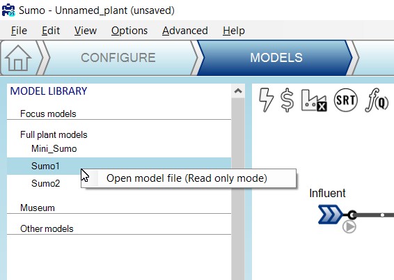
Table 3.2 lists the main processes included in the Sumo whole plant model family.
Table 3.2 – Main processes included in Sumo whole plant models
|
General full plant models |
Focus models |
|||||
|---|---|---|---|---|---|---|
|
Mini_Sumo |
Sumo1 |
Sumo2 |
Sumo2S |
Sumo2C |
Sumo4N |
|
| COD removal |
X |
X |
X |
X |
Two populations: OHO and AHO |
X |
| EPS production |
|
|
|
|
X |
|
| Denitrification |
1-step |
1-step |
2-step |
2-step |
2-step |
4-step |
| Hydrolysis |
X |
X |
X |
X |
X |
X |
| Fermentation |
X |
X |
X |
X |
X |
X |
| Anoxic methylotrophs |
|
X |
X |
X |
X |
X |
| Nitrification |
1-step |
1-step |
2-step |
2-step |
2-step |
4-step |
| EBPR (PAO-GAO model) |
|
X |
X |
X |
X |
X |
| Three-population anaerobic digestion |
X |
X |
X |
X |
X |
X |
| Temperature sensitivity |
X |
X |
X |
X |
X |
X |
| Precipitation |
|
X |
X |
X |
X |
X |
| Chemical P removal |
based on ASM2d approach |
Kinetic approach |
Kinetic approach |
Kinetic approach |
Kinetic approach |
Kinetic approach |
| Sulfur cycle |
|
|
|
X |
|
|
| GHG emissions |
|
|
|
|
|
X |
Important comment on Mini_Sumo: unlike other Sumo whole plant models, Mini_Sumo does not include colloidal components. The user should pay careful attention on the influent fractionation and – if required – primary clarifier calibration, so that the primary effluent composition in term of BOD and TSS is in agreement with the expectations.
Note: other models may be available as add-ons. Please write to support@dynamita.com for information.
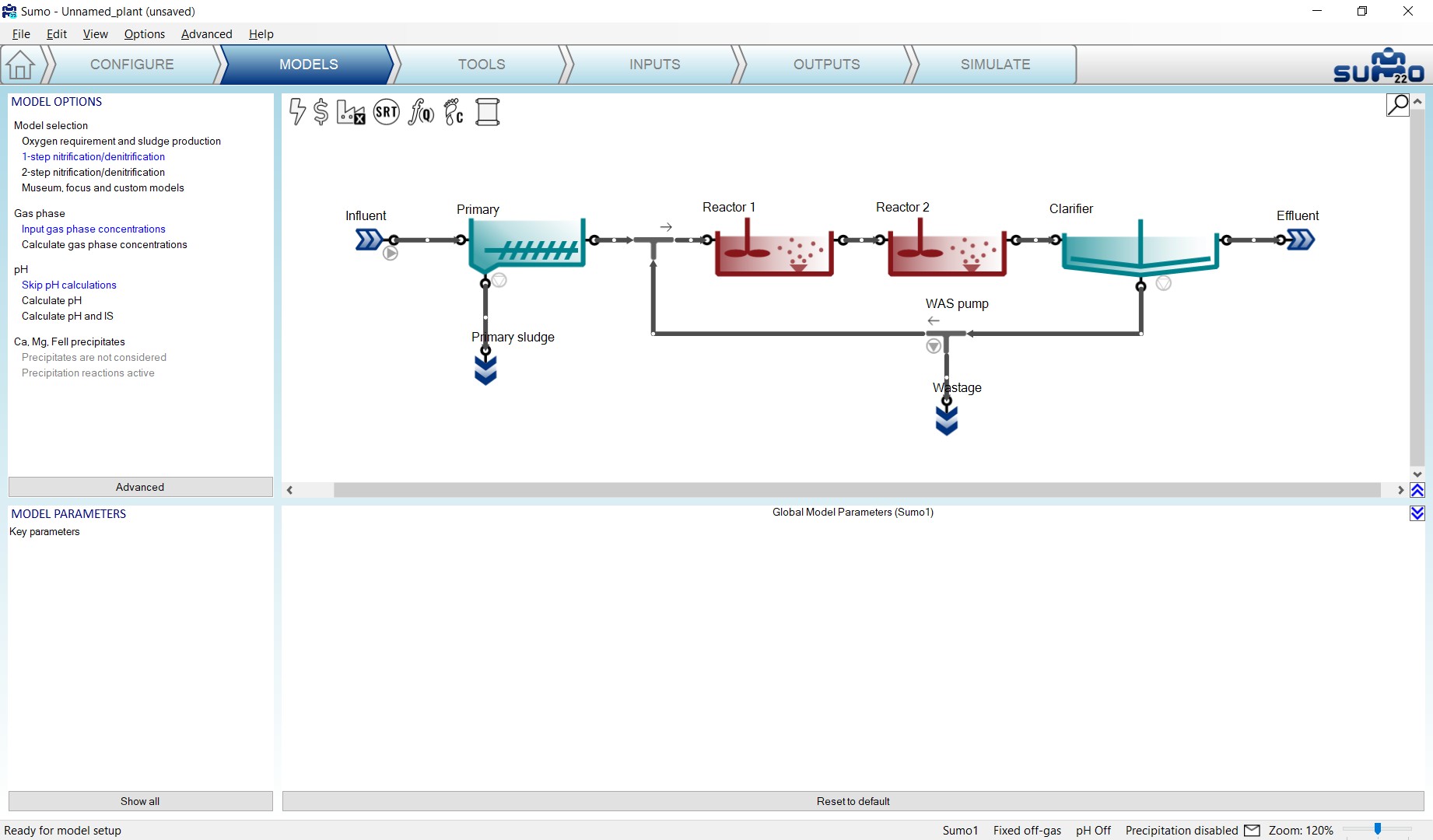
In our example we will use the default model setup with one step nitrification-denitrification model (Sumo1) with specified input gas concentrations (gas transfer is approximated, off-gas concentrations are fixed) and without pH calculation (therefore chemical precipitation is not calculated either), as shown in Figure 3.8.
¶ Global model parameters
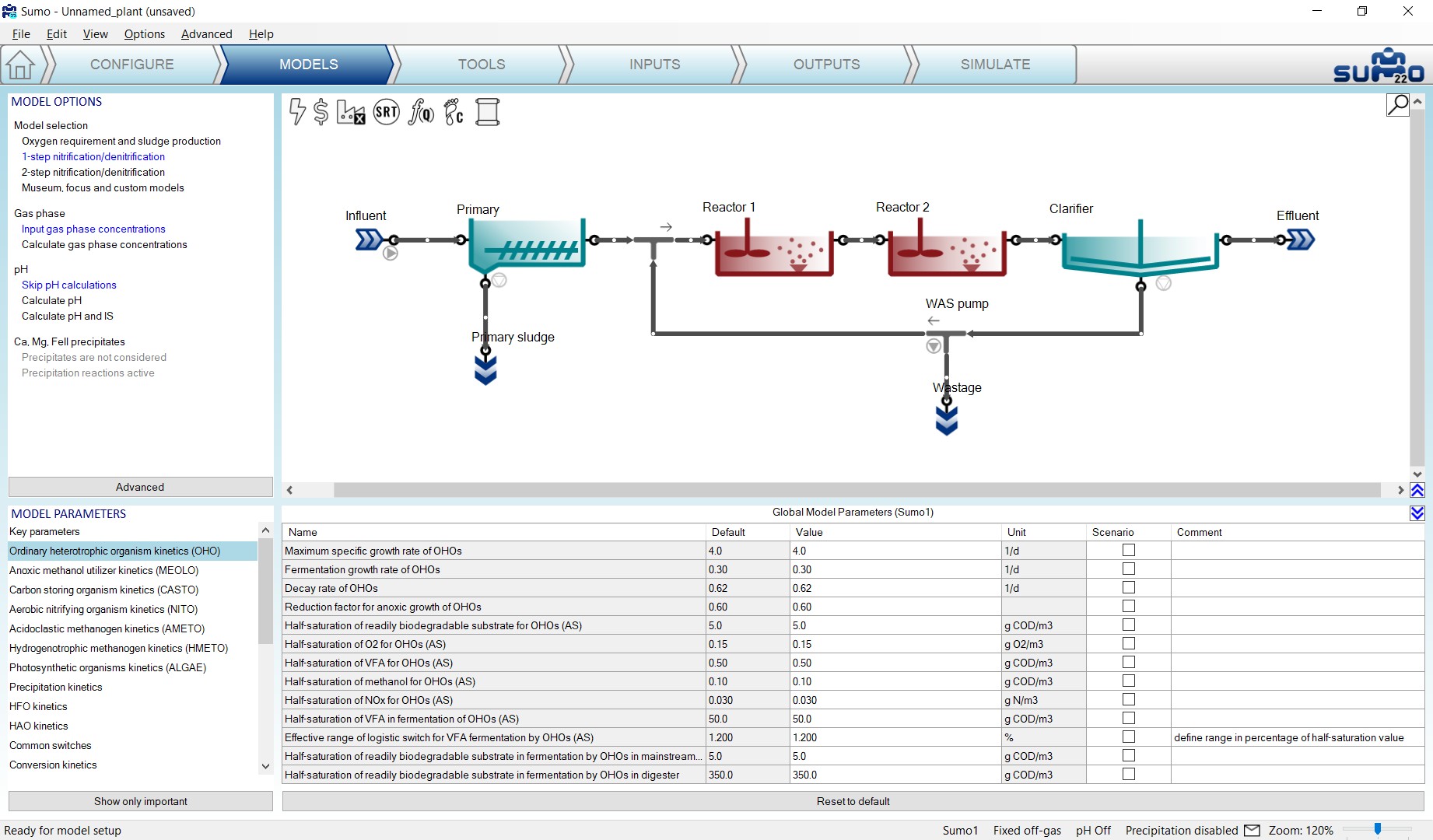
On the Models tab, if none of the process units are selected, clicking on the parameter categories listed in the bottom left panel (remember to click the Show all button in order to access all parameter tables in Sumo models), global kinetic and stoichiometric model parameters can be reviewed/modified. Each table will open up in the bottom right panel. This way the model parameters can be set globally, for the whole plant (Figure 3.9). These parameters will not be changed in this tutorial.
¶ Local model parameters
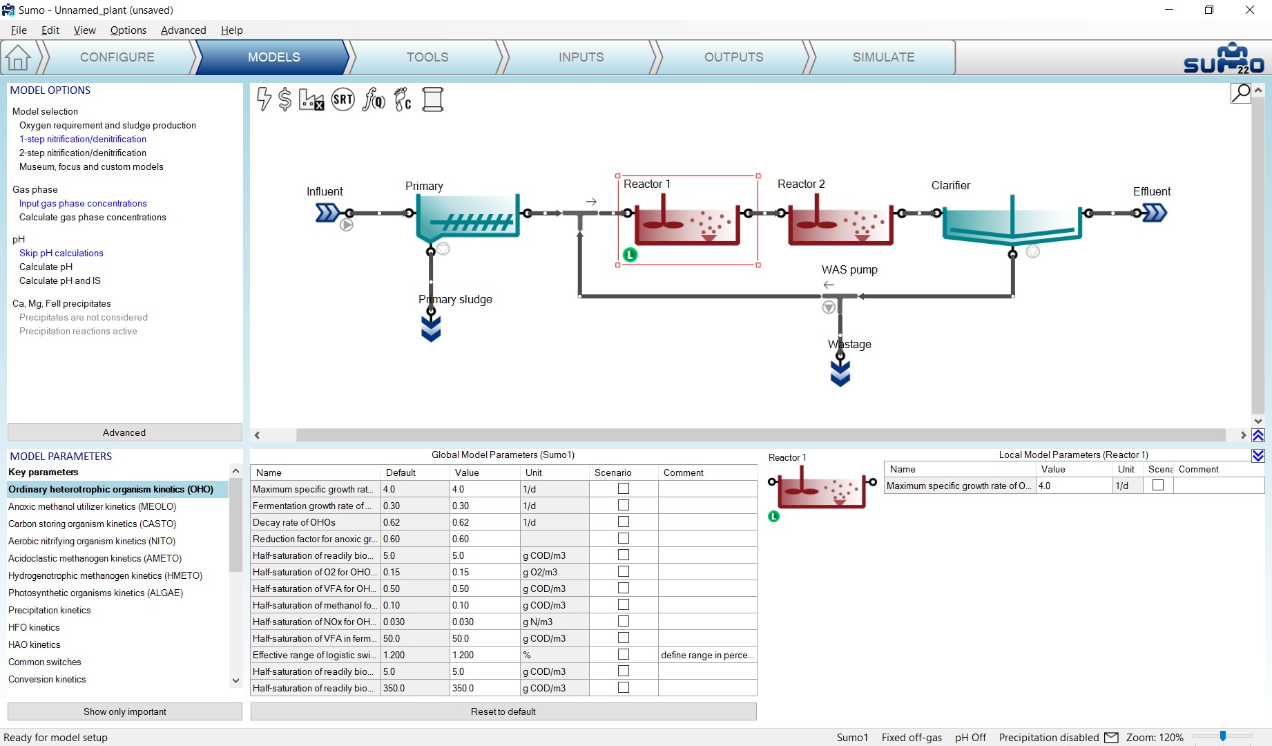
Any model parameter can as well be set as a process unit specific “local parameter”, by selecting the unit and dragging the desired parameter to the right side of the bottom right panel, as shown on Figure 3.10. In this case, the process unit will get a green “L” mark to remind the user for the local changes. Local model parameters will NOT be used in the current example, the aim of the above description was to explain this advanced functionality. You can remove local parameter selection by right clicking on the name of the parameter and selecting Remove.
¶ Tools
Proceeding to the Tools tab, complex plantwide calculations can be defined (Figure 3.11).
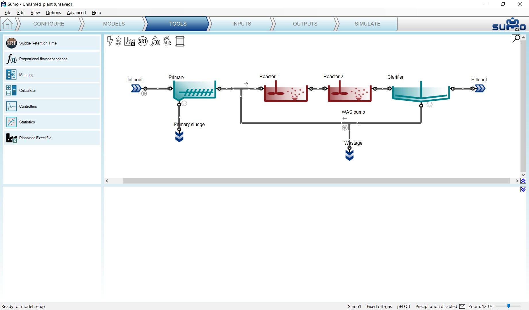
“Plantwide” means that the calculations are based on variables contained in several process units around the plant. The following calculations can be added to the simulation (listed in the top left panel):
- Sludge Retention Time
Plant specific SRTs (total, aerobic, etc.) can be calculated.
- Proportional flow dependence
Plant specific flow dependence (e.g. RAS flow as percentage of influent flow) can be defined.
- Mapping
Parameters can be mapped from one process unit to another one.
- Calculator
Variables (e.g. volumes, masses) can be summed up in the plant. Simple and advanced variable ratios can be defined for the plant (e.g. N removal efficiency = effluent TN/influent TKN).
- Controllers
Controllers allow the user to configure automatic control (such as time based on/off, PID etc.) of process unit parameters.
- Statistics
A few statistical options (Moving average, Noise generator, Totalizer ) are available here.
- Plantwide Excel file
The plantwide code is not confined to one process unit (PU) but can use variables from all over the plant model. The plantwide code file can be opened from the GUI directly. Further information and an example can be found in the Technical Reference document.
¶ Sludge Retention Time
The SRT calculation is set up the following way: drag reactors that contain sludge mass to the numerator and drag wastage – and if desired, effluent connections (ports) – in the denominator, as illustrated by Figure .
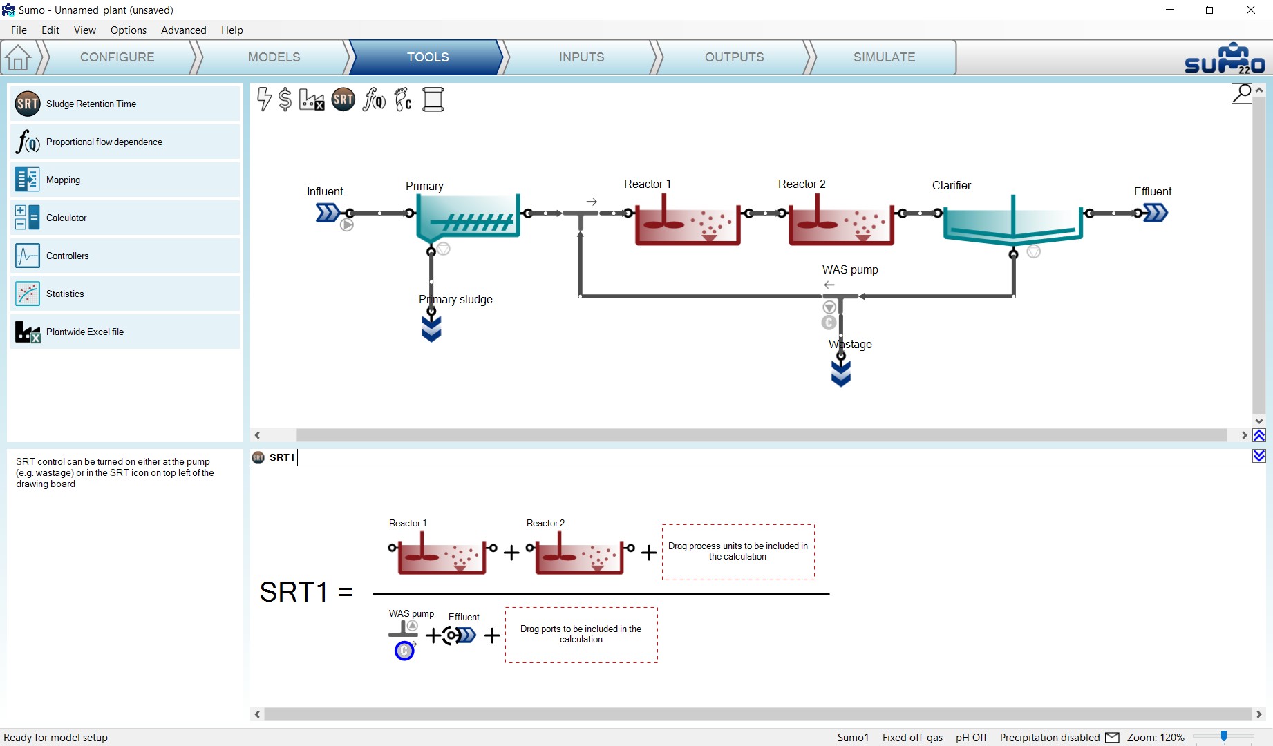
Several SRT calculations can be set up, e.g. total and aerobic, or North and South side SRT, etc. In this tutorial the total plant SRT will be calculated (as shown on Figure 3.12).
Note: When the project has an SRT calculation, the SRT icon on top of the drawing board gets a brown color.
Target SRT can be defined as well, by assigning a proper controlled port. These ports, such as the WAS pump in our example, are indicated by a “C” sign within a blue circle. A certain pump can only be used to control one SRT. Pumps can be selected and deselected for SRT control by right clicking their icon in the equation and choosing the desired option. When a pump is selected for control, Remove Controlled will deselect it (the “C” sign will disappear from the blue circle), while non-controlling pumps can be set to be controlling ones by choosing Mark as Controlled (Figure 3.13).
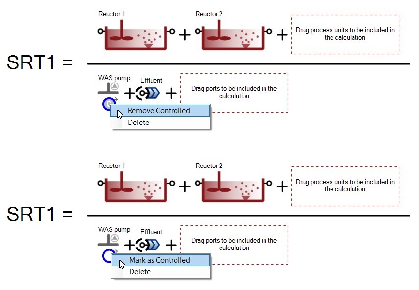
Note that even though the wastage pump is selected for SRT control, it has not been designated yet for this role at the current stage (this is indicated in the plant layout by a grey “C” sign next to the pumped outflow pipe of the WAS pump). The activation of the SRT control can take place in a subsequent step (see the Plantwide inputs chapter).
¶ Sum of variables
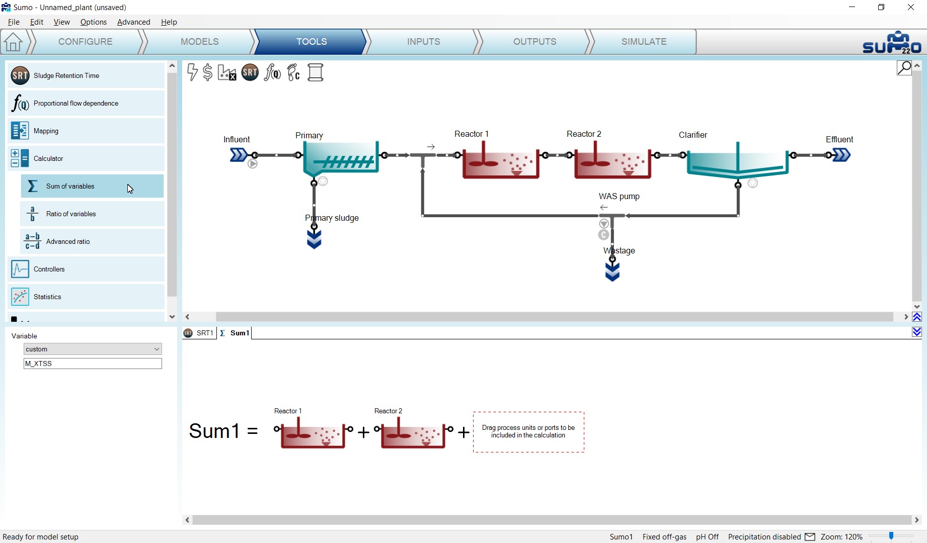
For calculating the Sum of variables, a set of predefined items are available (organized into groups) from dropdown menus in the bottom left panel. If the desired variable cannot be found here, custom variable input can be used well (choosing the last item in the first dropdown menu). In the latter case, make sure that the correct symbol is used, otherwise the built-in GUI check will disallow the calculation. Symbols of variables can be figured out using various methods (hints will be given in a subsequent chapter; details of the naming convention are described in the Technical Reference).
In this example, we will calculate the sum of Suspended solids mass in the reactors by entering “M_XTSS” as custom variable and dragging Reactor 1 and Reactor 2 into the equation from the layout (Figure 3.14).
¶ Ratio of variables
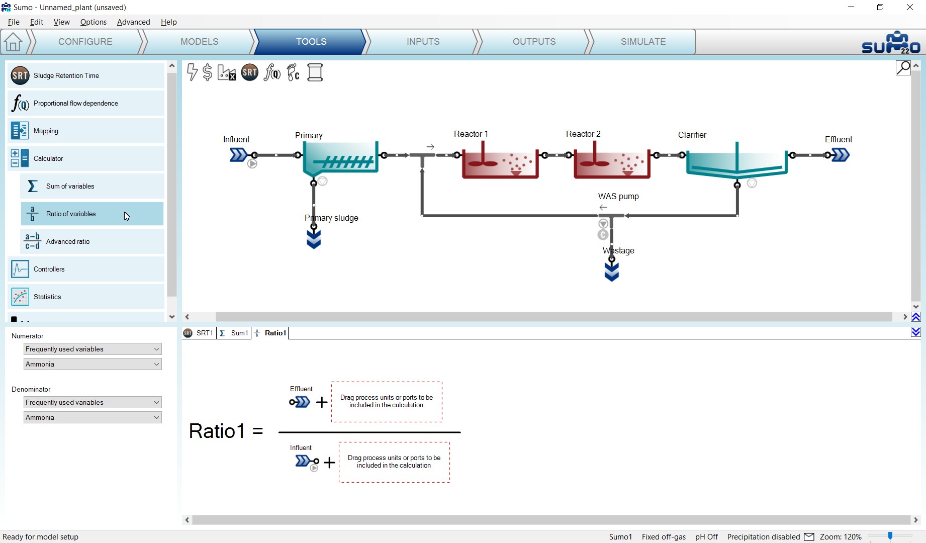
Adding Ratio of variables can be done in a similar way as the Sum of variables. First select the variables to be used in the numerator and the denominator from the dropdown lists of the bottom left panel, then drag the desired process units to the ratio. In this example, we will calculate the removal ratio of Ammonia, as shown on Figure 3.15.
¶ Proportional flow dependence
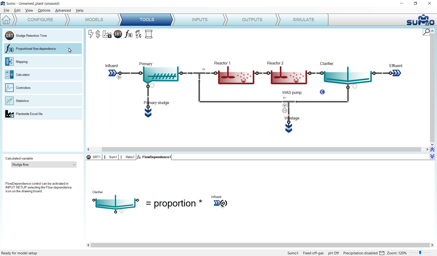
Adding Proportional flow dependence can be done by dragging the desired process units to the respective slots of the dependence equation. In this example, we are going to set the clarifier sludge recycle flow to be proportional to the influent flow rate, as shown on Figure 3.16. You will see a blue “C” sign showing up beside the clarifier on the drawing board, indicating that its sludge flow became a dependent parameter (controlled by the influent flow). The exact value of the proportional dependency will be set in a subsequent step (see the Plantwide inputs chapter). The controlling flow (e.g. influent) must not be within the loop (i.e. 50% of clarifier input flow to set the RAS flow cannot work as there is no solution to that loop).
Note: When the project has a proportional flow dependency, the “Q” in the f(Q) icon on top of the drawing board gets a blue background.
¶ Controllers
Controllers help to keep certain operational parameters of the selected process unit at a required setpoint or within a band. The following controllers are integrated into Sumo22 (Figure 3.17).
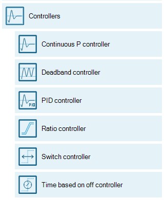
In this example, we will use a Deadband controller to control the sludge wastage pump automatically, in order to maintain the MLSS between certain limits. Details about the further controller options can be found in the Controllers chapter.
¶ Deadband controller
Adding a Deadband controller can be done in a similar way as the Sum of variables. First drag and drop the manipulated unit to the left side of the equation in the bottom right screen panel, and then the controlling unit to the right side of the equation. In the bottom left screen panel, you can now select the control variable (CV) and the manipulated variable (MV, a parameter) of the selected units. In this example, we will manipulate the Wastage pump to achieve the desired MLSS range, see Figure 3.18. Note that the “C” sign by the wastage pump will change to blue color, indicating that we have just set up and designated a controller for it that took over the role of the previously defined (but not activated, hence the former grey color) SRT control.
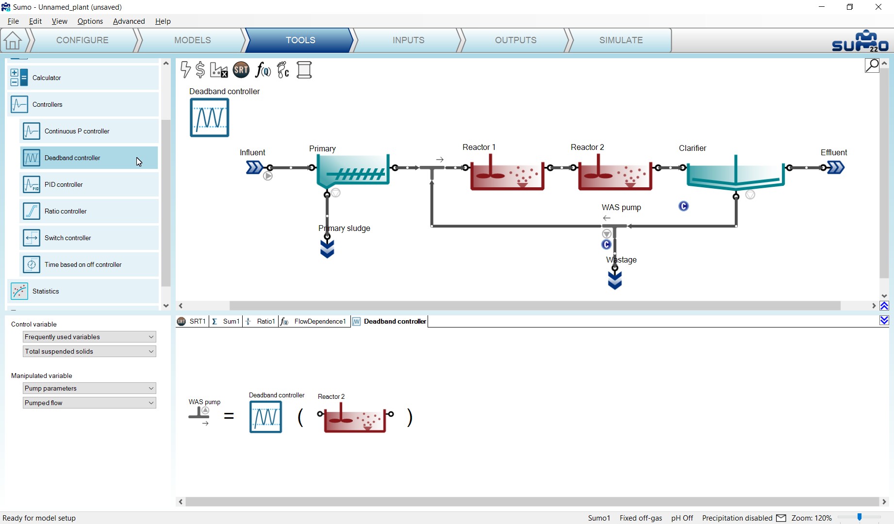
The controller image that appears in the plant layout can be repositioned on the drawing board by holding the CTRL key while the icon is being dragged and moved, so the layout can be better understood. Move the controller icon above Reactor 2, then select it and hit F2 (or alternatively, right click on the tab header in the bottom right panel) to rename it to “MLSS control by WAS”. This will rename the respective tab (or the controller icon) as well.
¶ Statistics
The Statistics section contains calculations for easier understanding or presentation of the results, such as average or totalized calculations. The following statistical calculations are integrated into Sumo22 (Figure 3.19).
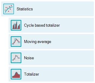
As an example, we will set up the average effluent concentration of the plant.
¶ Moving average calculation
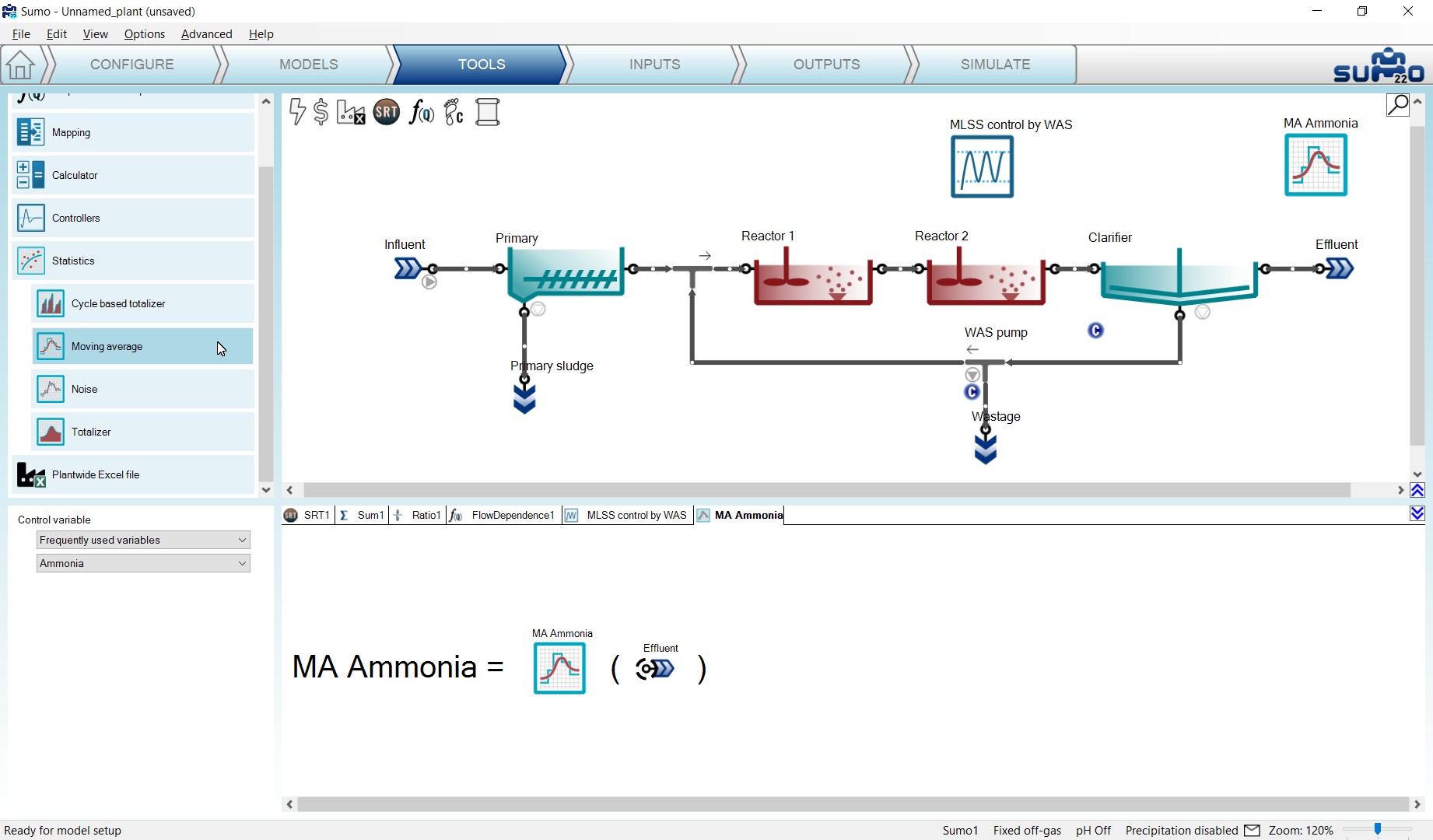
Moving average can be added in a similar way as Sum of variables. First drag and drop the process unit to which the calculation should apply, to the right side of the equation on the bottom right panel. In the bottom left panel you can now select the desired variable whose average should be calculated. In this example we will calculate the average effluent ammonia concentration, see Figure 3.20.
The statistical unit image can be repositioned on the drawing board and renamed similarly to controllers. Move the icon above the Effluent and rename it to “MA Ammonia”.
¶ Inputs
Choosing the Inputs task, the blue workflow tab above the drawing board automatically splits into Constants and Dynamics. According to this, different types of settings become available: we can set either constant inputs (e.g. fixed influent composition, reactor DO setpoints etc.) or dynamically changing inputs (e.g. variable influent flow, composition, shifting reactor DO setpoints etc.). At this point, Sumo will be compiling your model in the background (you can track the progress in the Status Bar). However, in most cases, you can already start providing information to Sumo. When your layout requires using arrays (e.g. layered clarifiers, biofilm), please wait until the model is fully compiled and loaded (status bar message: “Ready for Simulation”). For the initial plant setup, we will only need the Constants, as shown on Figure 3.21. Select each object one by one and enter the required values as shown below.
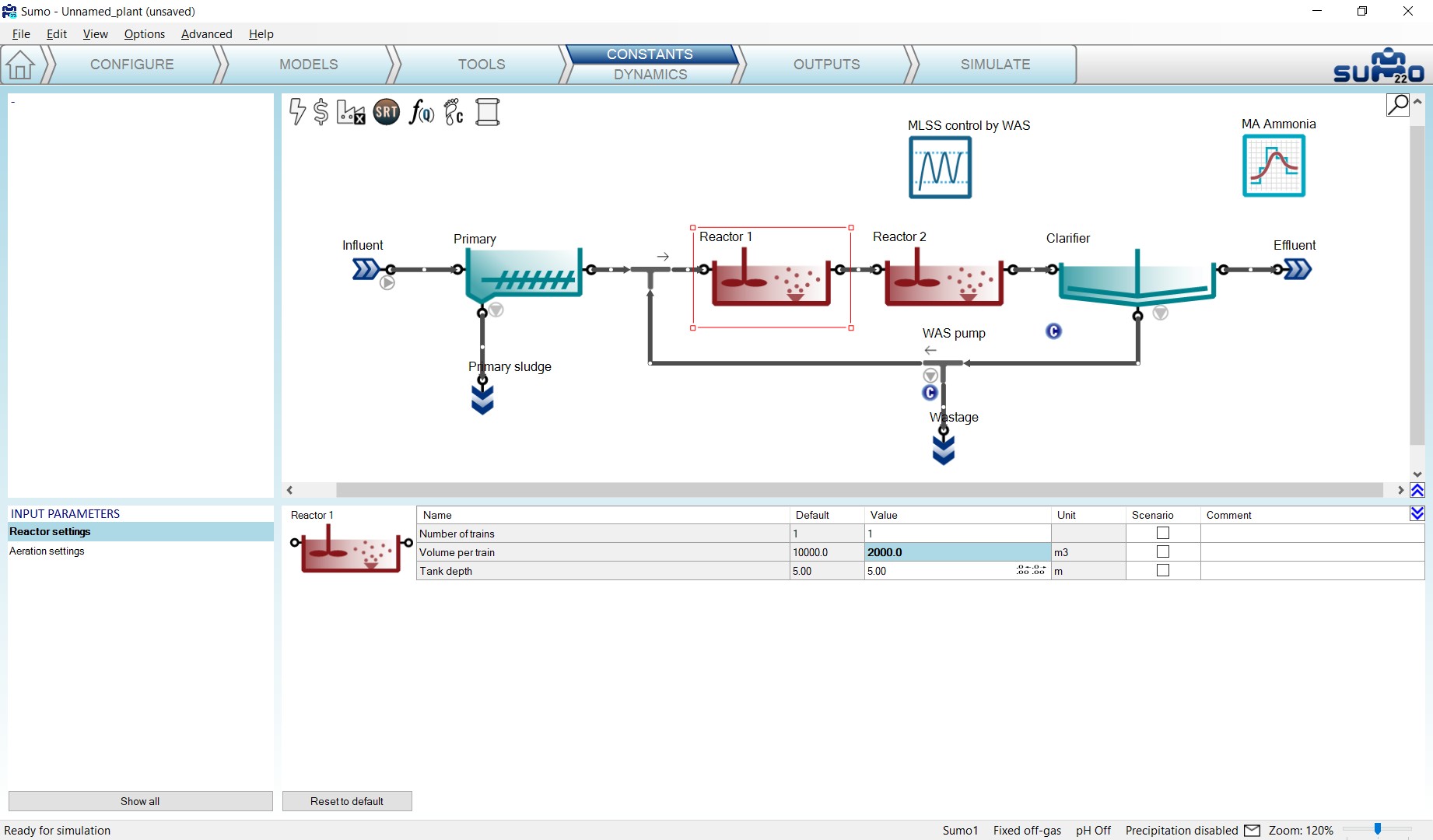
In this simple configuration, we only need to set a few values to build a realistic plant model, first for typical dry weather operation. Use the values from Table 3.3 for this example (leave everything else at default):
Table 3.3 – Input setup for AS plant
| Process Unit | Parameter group | Parameter | Value | Unit |
| Reactor 1 | Reactor settings | Volume per train | 2000 | m3 |
| Reactor 2 | Reactor settings | Volume per train | 8000 | m3 |
| Influent | Influent specifications | Flow rate | 20000 | m3/d |
| Influent | Influent specifications | Total COD | 500 | g COD/m3 |
| Influent | Influent specifications | Temperature | 22 | °C |
Enter these values by selecting the respective process unit on the drawing board and the parameter group in the Input parameters menu (bottom left panel) – the values can be edited in the bottom right panel (Figure 3.22). Each value that is different from the default will be highlighted with bold letter type. There is also a similar indication in the Input parameters menu for parameter groups that contain non-default values.
Whenever the entered value is out of the allowed range specified in the model, Sumo will notify you with a prompt window and set the value to the nearest feasible bound, indicating the automatic choice by applying red color to the text. This value can be overridden manually with a valid number.
If needed, all changes applied to the values of the actual parameter group can be reverted to defaults by clicking the Reset to default button located in the bottom right screen panel (Figure 3.22). Also, there is a unit conversion module for US units (MGD, scfm, etc.) in the Options menu item if needed.
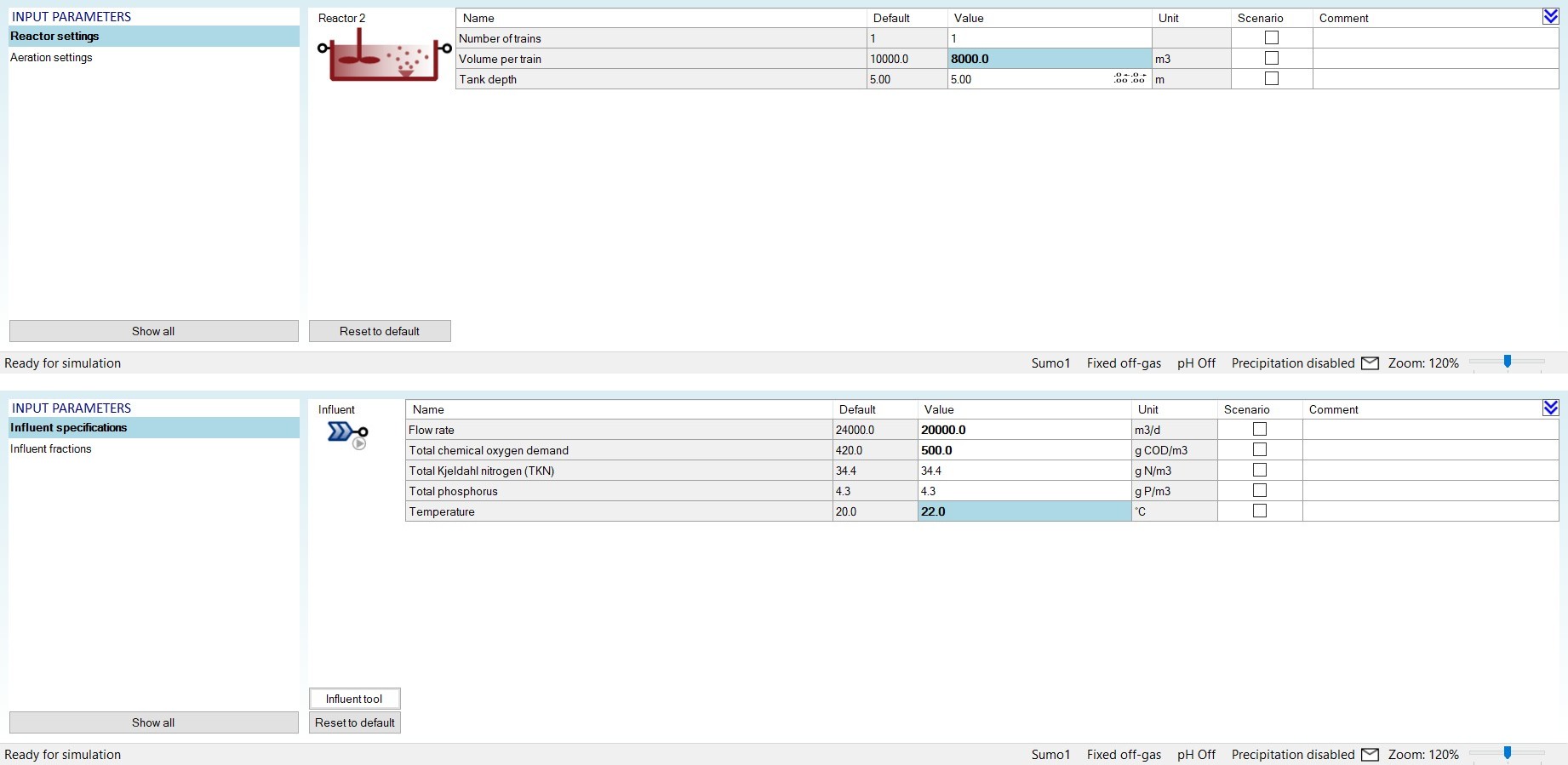
For setting the plant specific influent composition, the use of the Influent tool Excel file is recommended. The Influent tool can be reached directly from the input setup of the Influent, by clicking the button located in the bottom right screen panel (Figure 3.23).The details of the Influent tool are described in the Influent tool chapter. At this point, we will not alter the influent composition, so we will skip using the Influent tool.
Parameters for scenario analysis can be selected by using the checkboxes in the Scenario column. In this example, we will select the influent flow rate, total COD and the temperature (Figure 3.23). The use of scenarios will be described in the Scenarios chapter.

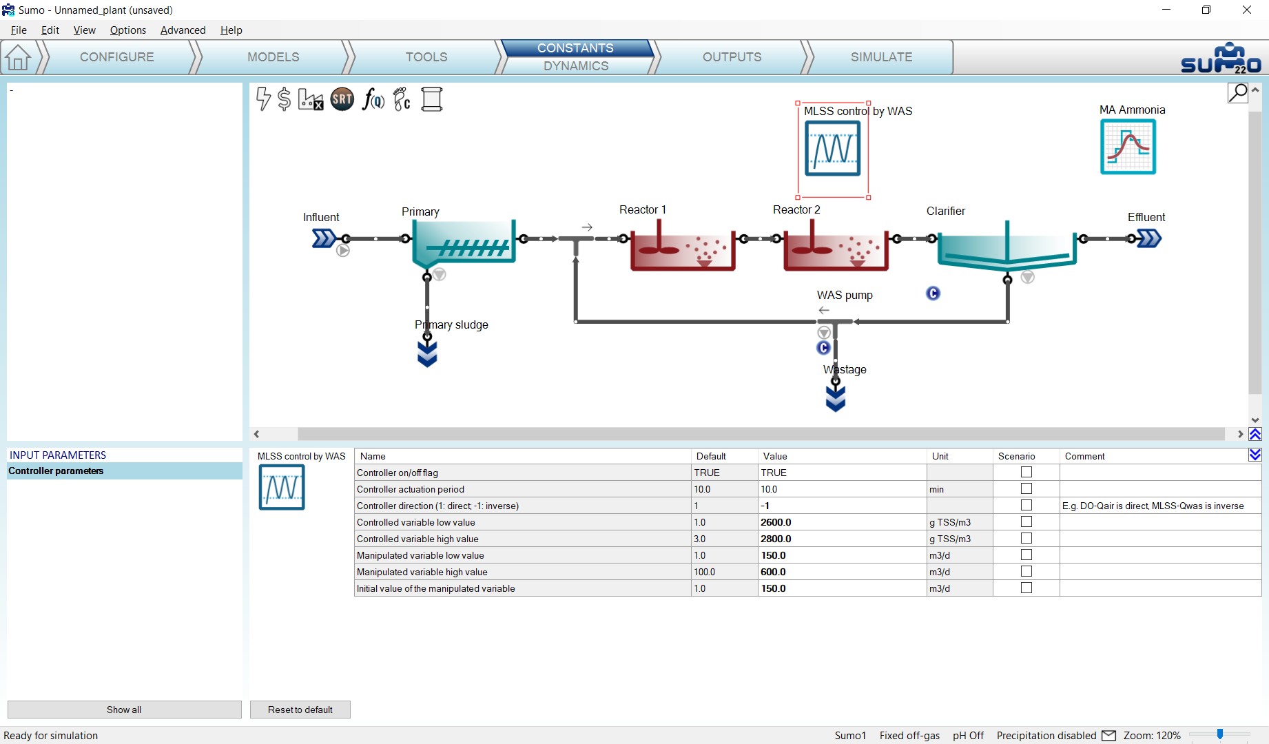
The controller parameters can be setup at this stage as well. In this Deadband controller example, we will set:
- Controller direction: inverse (-1), since increasing wastage (MV) will decrease MLSS (CV), i.e. the CV responds inversely to MV change;
- 2600 mg/L as low value and 2800 mg/L as high value for the Controlled variable (MLSS in Reactor 2) range;
- 150 m3/d as low value and 600 m3/d as high value for the Manipulated variable range (the latter represents the physical pump capacity for the Wastage pumped flow);
- Initial value of manipulated variable to single pump capacity as 150 m3/d.
See these settings on Figure 3.24.
The input setup of this wastewater treatment plant model is now ready.
¶ Influent tool
The Influent tool is a multiple sheet Excel file to help to set up the proper influent composition. The role of each sheet is explained in Table 3.4 below.
Table 3.4 – Description of the Influent tool
| Influent tool sheets | |
|---|---|
| Help | Short description of the file content |
| Data | Input of the available measurement data of the simulated plant or facility. This sheet provides help to estimate the missing data based on available information for municipal or industrial wastewater composition. |
| Check fractions | On the left side of the sheet, the estimation of key organic fractions is available, such as COD and N fractions, particulate COD/VSS ratios by component, yield on ultimate BOD and BOD fraction for soluble, colloid and particulate. On the right hand side, the calculated COD, BOD5 and TSS/VSS values can be checked if they match the measured values. |
| Sumo forms | This sheet gathers all the information that can be used to simply copy into the Sumo Models or Inputs tab of the Influent process unit. |
| Fractionation tree | This sheet shows the fractionation graphs of total COD, suspended solids, N and P based on your input data, helping to visualize the organization of the individual fractions used in the model. |
| Balances | On this sheet, the organic compounds can be checked (how the fractions add up to the total). The sheet will also provide warning when negative component concentrations result from the estimated fractions (such as not enough N for organic TKN if most of TKN is ammonia, and there are solids in the influent) |
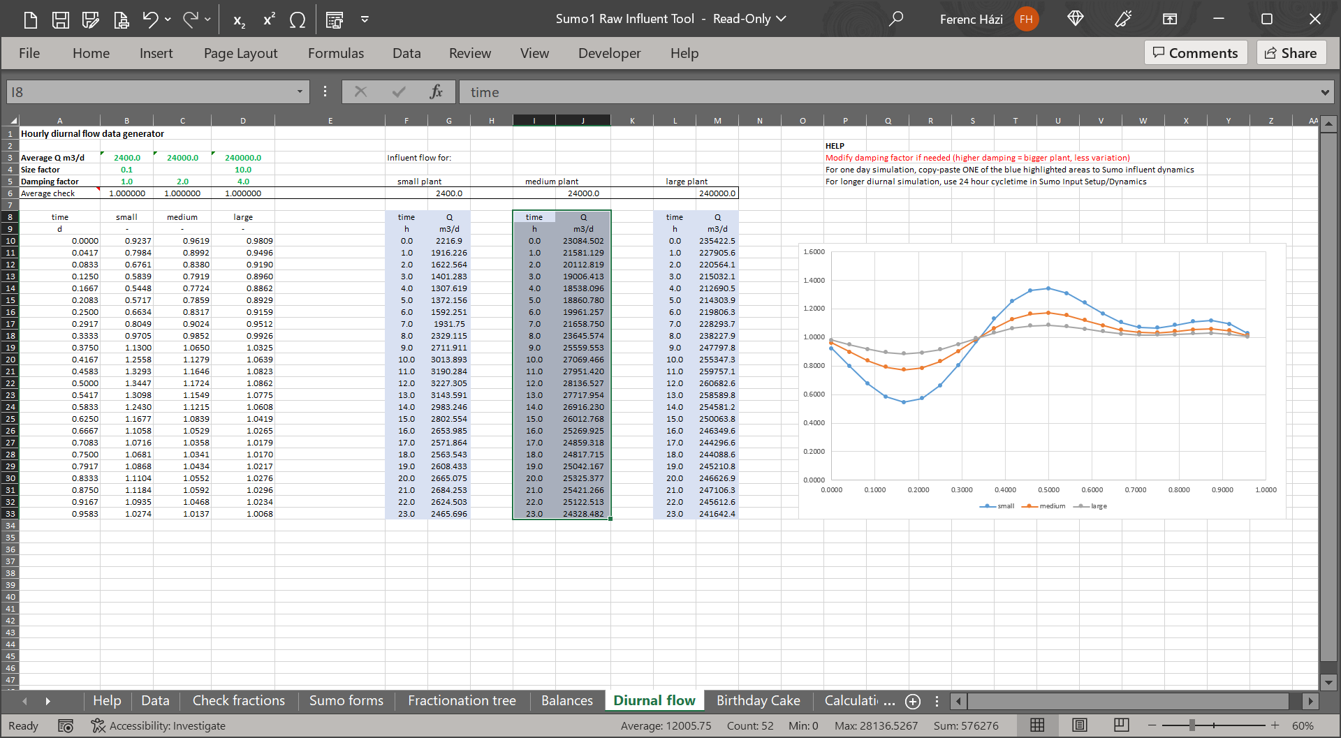
| Diurnal flow | This sheet provides example and usual flow pattern for small, medium and large plants. Based on the influent value, the diurnal flow dynamic input tables are prepared for copy and paste into Sumo. |
| Birthday cake | On this sheet, you will find a ready-made table for a “birthday cake” type of load analysis, prepared from your input and diurnal flow data. |
| Calculations | This sheet contains the details of BOD calculation and the error tolerances used on Check fractions sheet. |
For a detailed description of the Influent tool please refer to the Tools in Sumo chapter of the Technical references, and guidelines for influent fractionation are available in Influent characterisation chapter.
¶ Dynamic Inputs
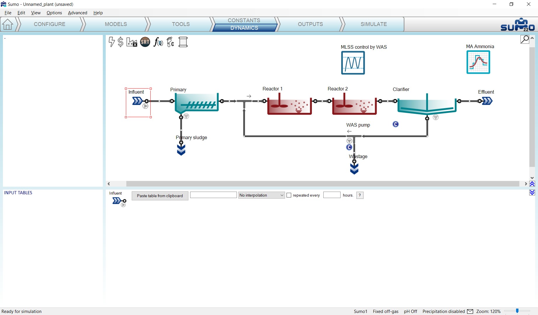
This optional task can be used to enter dynamically changing input information, e.g. diurnal flows, DO schedules and more. To activate the dynamic input setup, click on the lower part of the Inputs tab on the Task Bar, labeled as Dynamics.
The role of screen panels in Dynamic Inputs mode are the following:
| Top right panel | Plant configuration |
| Top left panel | Unused in this mode |
| Bottom right panel | Data entry functionality |
| Bottom left panel | List of entered dynamic data tables |
If we wish, we can copy and paste entire data tables from an Excel file into Sumo. This will be discussed later in the Subjecting the plant to dynamics chapter.
¶ Plantwide inputs
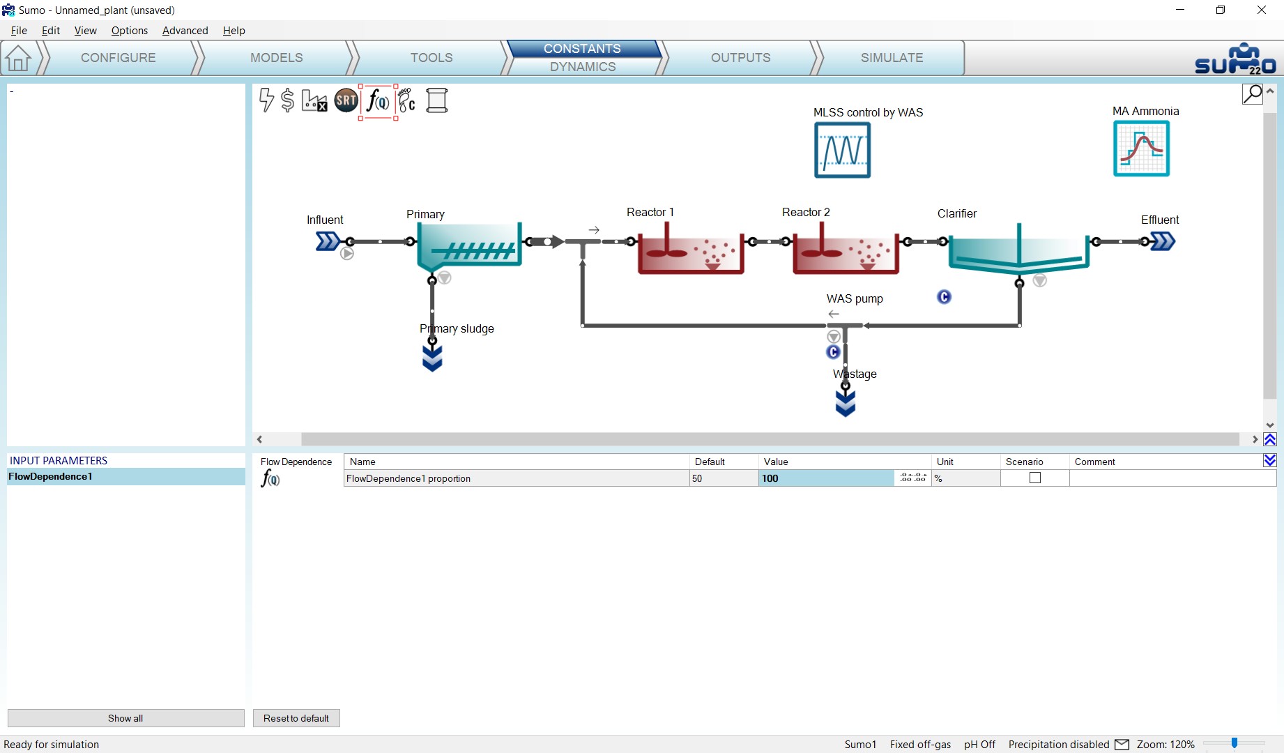
Target SRT and proportional flow dependence input settings can be accessed by clicking on the respective icons listed on the top left part of the layout panel. In this simulation, we will not use the Target SRT controller, but will set up the proportional sludge flow of the clarifier to 100%, as shown on Figure 3.26. This will align the sludge flow rate with the influent flow as 1 to 1.
The plantwide parameters set in the Plantwide Excel file will appear in the Inputs tab when the plantwide (factory) icon is selected in the top section of the layout. These can also be changed dynamically, similarly to any other model parameter (for more detailed information on this feature, please consult the Technical Reference). In this simulation, we will not use plantwide parameters.
¶ Outputs
This task can be used to specify which variables and in what format should be displayed and/or saved during the simulation phase (Figure 3.27).
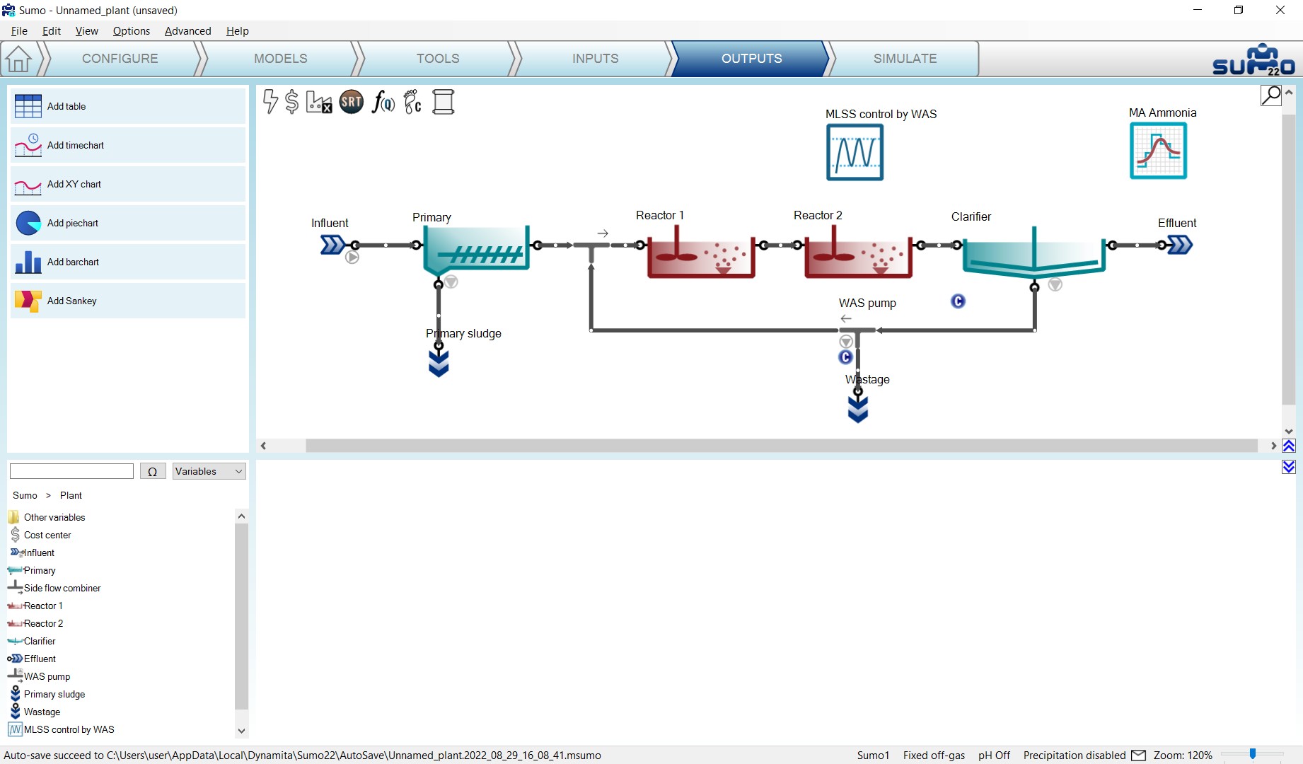
The role of screen panels in Outputs mode are the following:
| Top right panel | Plant configuration |
| Top left panel | Buttons for different diagram types (Table, Timechart etc.) |
| Bottom right panel | Added outputs in a series of tabs |
| Bottom left panel |
Output variable list for the selected unit and the connected pipes Available once the model is fully compiled. The user can browse the variables based on their name or symbol. There are also preselected categories (frequently used, operational variables etc.) available to help the work. |
¶ Adding a table
Click the Add table button in the top left panel: this will add a table to the bottom right panel. The table can be renamed (right click on the tab and choose Rename from the pop-out menu or simply just double-click on the tab) and several tables can be added. Name this table “Results”. Add process units to the table by dragging them to the table (by selecting multiple units in the drawing board, they can be added in one go as well). Add variables to the table by selecting and dragging them from the bottom left panel (Figure 3.28). Entire display tables can be added at once by dragging the prepared table e.g. Frequently used variables (Note: if the table has not been renamed by the user, it is automatically renamed when a whole display table is added). The exact list of preselected variables varies according to the process units (in this example, the Influent was selected when adding Frequently used variables to the table). Initial values will appear in the cells.
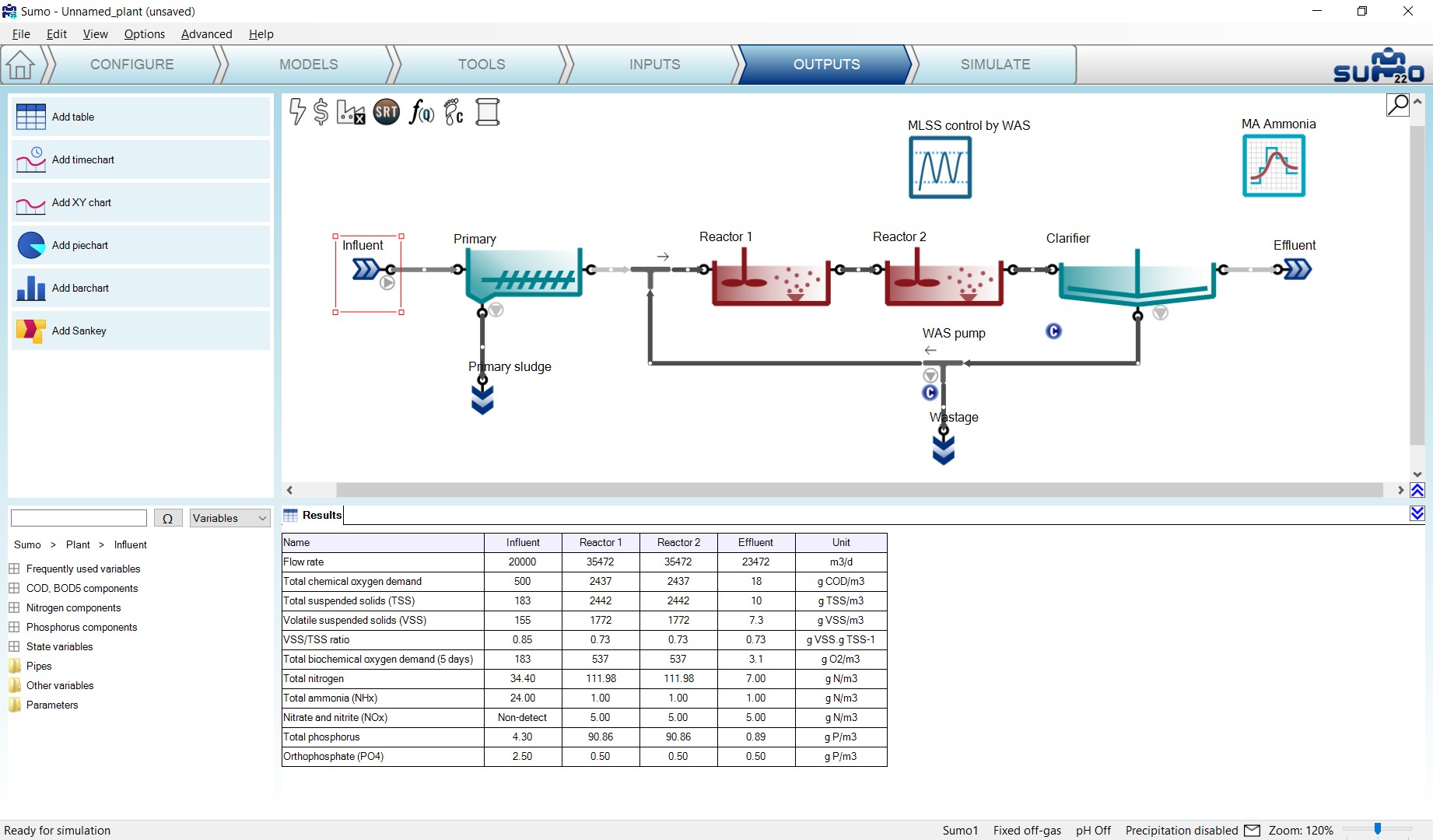
You can add also the DO and Offgas O2 content from the Frequently used variables of Reactor 1 (or 2).
Add another table and drag the Active biomass and Uptake rates for both reactors.
Note that the table columns (except for Name and Unit) can be reorganized by dragging the column header and dropping to the desired slot. Table rows can be rearranged likewise: first highlight the rows to be moved with the mouse, then drag and move the pointer out to the bottom left screen panel for a moment, and finally drop the rows to the desired new place. Units can be changed by clicking and selecting from the dropdown list. The number of decimal digits displayed can be customized to show meaningful detail by hovering the mouse over the numbers and clicking the respective icons – the action will apply to all numbers in the active table row.
¶ Adding a timechart
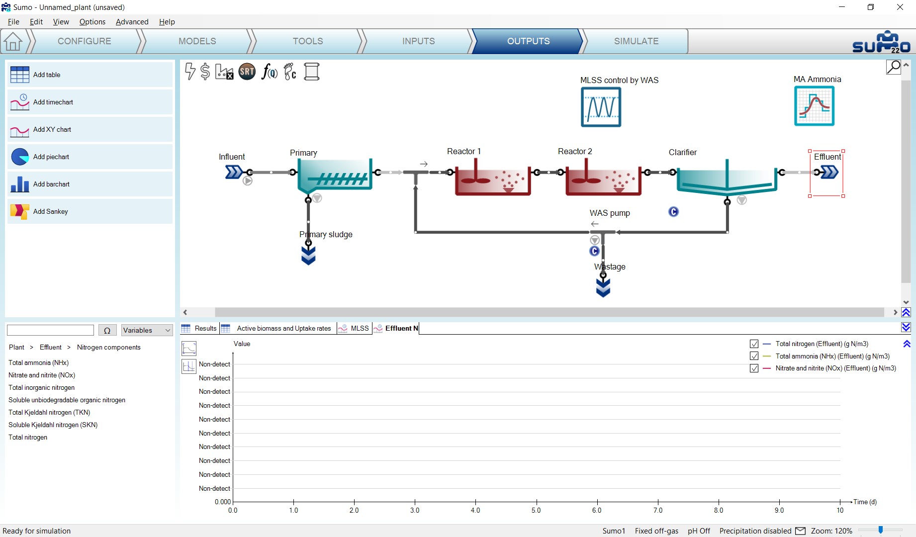
Click the Add timechart button in the top left panel: this will add a timechart to the bottom right panel as a new tab. Select a process unit on the layout and drag a variable from the bottom left panel on the timechart to be plotted (a legend will appear in the top right corner of the timechart). Several variables can be added to each timechart (new items will be appended to the legend), and several timecharts can be added as well (increasing the number of tabs). In this example we will plot MLSS in the reactors and wastage flow on one timechart (select the reactors one by one and add TSS from Frequently used variables); and effluent total nitrogen, ammonia, as well as nitrate and nitrite (available from Nitrogen components) on the second one (see Figure 3.29). Graphs will be plotted during the simulation phase.
¶ Adding an X-Y chart
This type of diagram can be used to demonstrate the relation between selected variables (e.g. equilibrium species) depending on another variable (e.g. pH). A practical application is shown in the example called Titration of ammonia solution.
¶ Adding a piechart
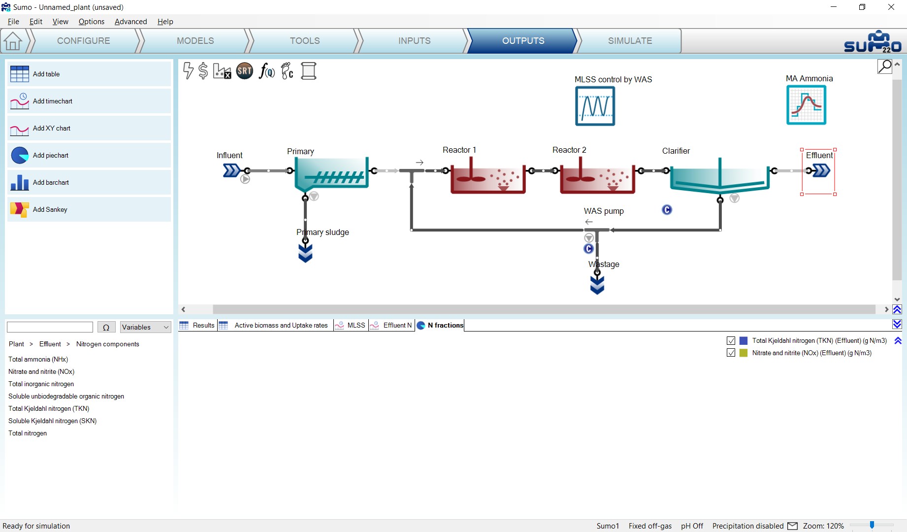
Click the Add piechart button in the top left panel: a new tab for labeled piechart will appear in the bottom right panel. Select the desired process unit on the layout and drag the variables to be depicted from the bottom left panel to the – yet empty – bottom right panel (a legend will appear in the top right corner). For this example, we will use Total Kjeldahl Nitrogen along with Nitrate and nitrite (available from Nitrogen components) in the effluent. Rename the tab to “N fractions” (Figure 3.30). The piechart will be rendered during the simulation phase.
¶ Adding a barchart
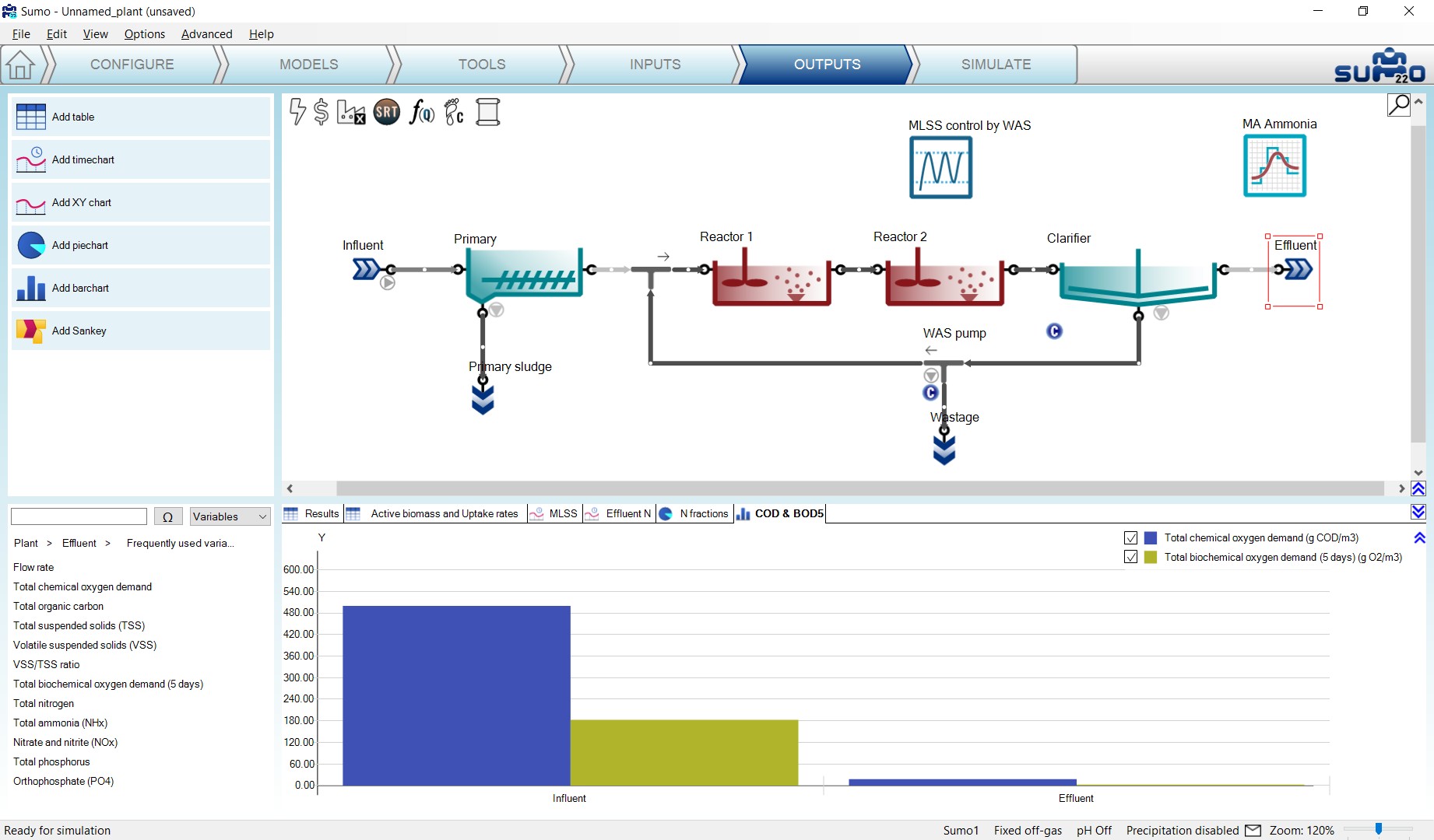
Click the Add barchart button in the top left panel: this will add a barchart to the bottom right panel as a new tab. Choose a process unit and drag variables from the bottom left panel to be shown on the barchart, just like in the previous chart types. Multiple variables can be added to each barchart, and several barcharts can be added as well. Dragging additional process units to the chart will add them with the actual set of variables and initial values will be shown. For this example, choose Total chemical oxygen demand and Total 5-day biochemical oxygen demand from the Frequently used variables in the influent and in the effluent (Figure 3.31). Rename the tab as “COD & BOD5”. The barchart will be continuously updated with the changes during the simulation phase.
Note that the order of process units in the barchart can easily be reorganized by dragging the name of the process unit and dropping it to the desired slot.
¶ Adding Sankey
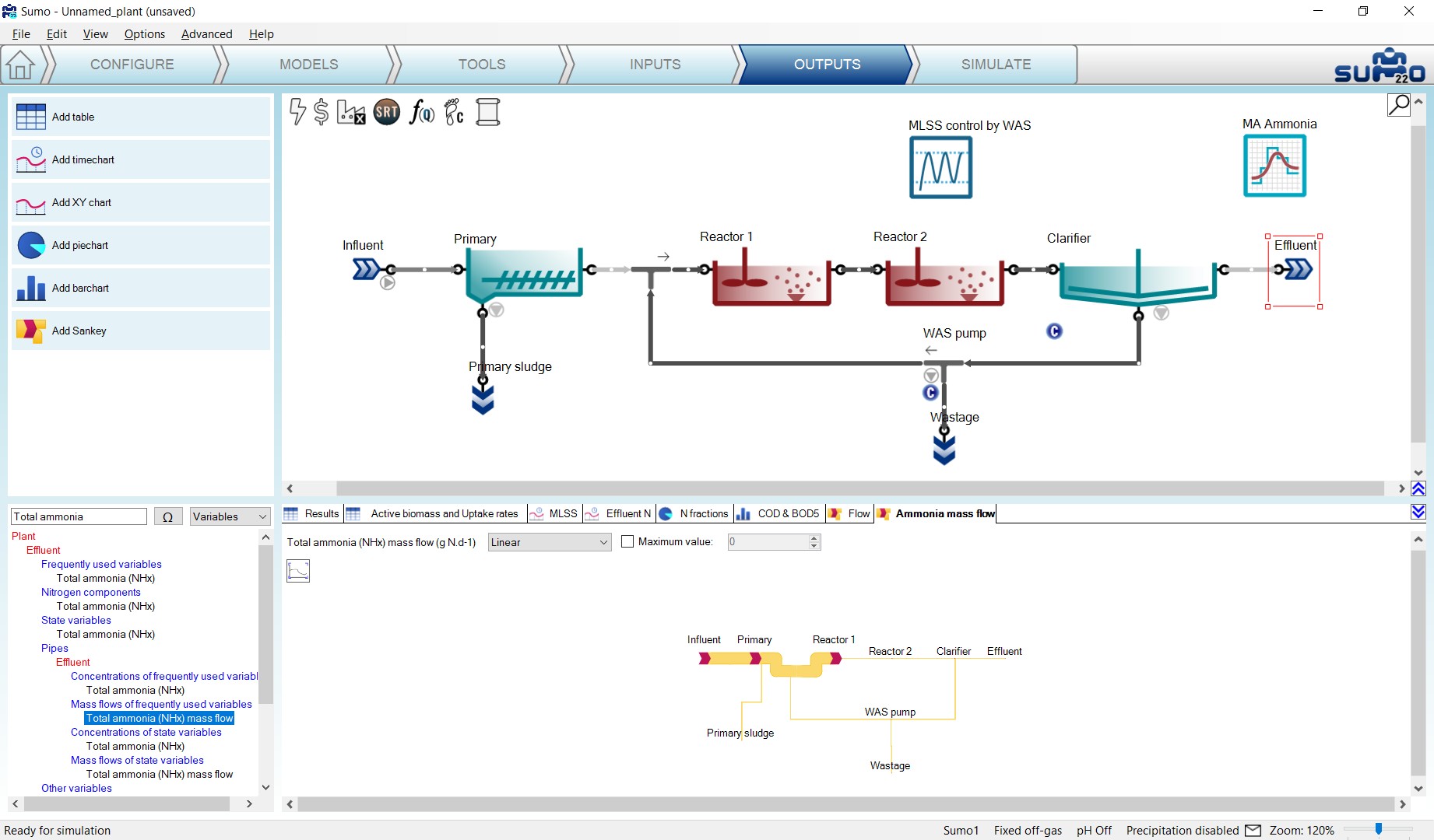
Click the Add Sankey button in the top left panel: this will add the Sankey diagram of flow by default. The variable can be changed by dragging any other item from the bottom left panel over to the bottom right panel. Several Sankey diagrams can be added, with one variable plotted on each Sankey. This example will use one Sankey with the default setting (renamed to “Flow”) and another one showing the mass flows of ammonia (renamed as “Ammonia mass flow”) as shown on Figure 3.32. Use the search field in the bottom left panel to find the latter: type in “Total ammonia” and locate “Total Ammonia (NHx) mass flow” under the “Mass flows of frequently used variables” list item in the search results. The search field works with all of the other output options as well.
At this point, the example is prepared for simulation with all the inputs and outputs provided. If desired, the output tabs can be reordered by dragging them to the aimed sequence. The file can be saved using the File menu (this function is not available in the demo version).
¶ Simulate
The last item on the Task Bar can be used to run simulations and observe the results.
The role of screen panels in Simulate mode are the following:
| Top right panel | Plant configuration |
| Top left panel |
Simulation control panel Different function buttons for the simulation, including report preparation in Excel format. |
| Bottom right panel |
Tabs for the previously defined outputs Display of results. |
| Bottom left panel | Tabs for scenario definition |
¶ Simulation Control Panel
The top left screen panel enables operating the model, to run dynamic or steady-state simulations (as well as algebraic calculations, when being in design mode). Steady mode can be used to calculate directly the steady-state condition of the variables, whereas Dynamic mode will show the variations with time.
¶ Steady mode
In systems theory, a system or a process is in a steady state if the variables which describe the behavior of the system or the process do not change with time. If a system is in steady state, then the recently observed behavior of the system will continue into the future.
After setting up the plant, all process units get a predefined initial value for each state variable (taken from the model defaults). However, most often this will not equal the values that can be observed in steady-state condition. The steady-state calculation will find the proper state variable values when the system is in steady state.
The steady-state simulation employs different solvers to look for the steady-state condition of the system. In this mode, all dynamic inputs are disabled and the controllers are turned into integrated controllers. Please note that steady-state simulation cannot be performed on inherently dynamic processes such as the SBR.
The roles of the control panel buttons on the Steady tab (Figure 3.33) are the following:
| Calculate Steady-state | Start steady-state simulation from current system state |
| Interrupt calculation | Interrupt simulation (or resume a previously interrupted one) |
| Reset | Reset the system to default initial conditions |
| Save plant conditions | Save actual conditions to a Sumo System State file |
| Load plant conditions | Load previously saved conditions from a Sumo System State file |
| Report | Generate a report in Excel format |
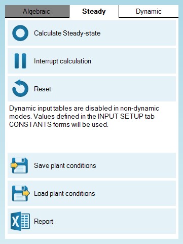
One should use the Reset button thoughtfully, especially when working with complex plants, for it will reinitiate the simulation with the default concentrations defined in the model and process units, and reaching steady-state again might be time-consuming in these cases. Saving plant conditions (especially if steady-state has been found) can be useful to restore system state in case the simulation is driven into an unwanted condition (e.g. accidentally having been reset).
¶ Dynamic mode
Dynamic simulation will follow changes within the system as time passes, starting from the actual state of the system, and applying all dynamic inputs and behaviors that were defined during the setup process.
The roles of the control panel buttons on the Dynamic tab (Figure 3.34) are the following:
| Start | Start a simulation from actual conditions |
| Steady-state start | Start a simulation from steady-state |
| Fast / Accurate | Choose between Fast and Accurate modes |
| Reset | Reset default conditions |
| Continue | Continue/Pause simulation |
| Stop time | Length of dynamic run |
| Data interval | Data plotting/updating interval |
| Save plant conditions | Save actual conditions to a Sumo System State file |
| Load plant conditions | Load previously saved conditions from a Sumo System State file |
| Report | Generate a report in Excel format |
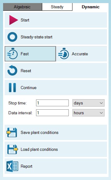
Dynamic simulation can be started by pressing the Start button. Upon first start, the simulation will be run from the initial conditions (defaults specified in the model file and in the process units). Every subsequent run will be initiated with the last system state. Pressing the Steady-state start button will run a steady-state simulation prior to starting the dynamic one (so that steady-state will be used as the initial condition). The role of the Reset button is the same as it is in the Steady mode – use it only if the goal is to restart the simulation process entirely from scratch.
The dynamic simulation will run until the end of the period defined by Stop time is reached (default setting: 1 day) and will plot/update results in the bottom right screen panel with the frequency described by the Data interval (default setting: 1 hour). The Stop time and Data interval can be modified before the simulation is started, or also when it is paused.
Choosing between Fast and Accurate modes translates to using different pre-configured solver settings. The differences between the two are described in Table 3.5. Usually the Fast mode is fast and accurate enough for most cases, and therefore its use is generally recommended. However, in certain situations (e.g. with biofilm models), the Accurate mode might provide faster simulation. If the plant seems to be complex and takes a long time to find a solution in Fast mode, then try switching over to Accurate. In such rare cases, it is the trial-and-error of coming to solver settings that lead to a speedy solution.
Table 3.5 – Explanation of Fast and Accurate solver settings
| Fast | Accurate | |
| Type of configuration | Simple plant layouts will provide a speedy simulation | Best for complex plant layouts, specifically which have biofilm processes (MBBRs, and trickling filters) and several return or recycle streams. |
| Solver types | GISA → Relaxation solver → Newton-Raphson | Relaxation solver → Newton-Raphson |
Note that the mode selection will also have effect on the steady-state solver: GISA introduces a strong perturbance to the system state, therefore it is quite suitable for finding steady-state from a distant initial system state, while not so necessary when the system is already close to steady-state. There is no difference however in the stop criteria for the solvers.
¶ A process simulation example – aerobic plant
The plant configuration we have just built is an aerobic plant, with 12-hour hydraulic residence time:

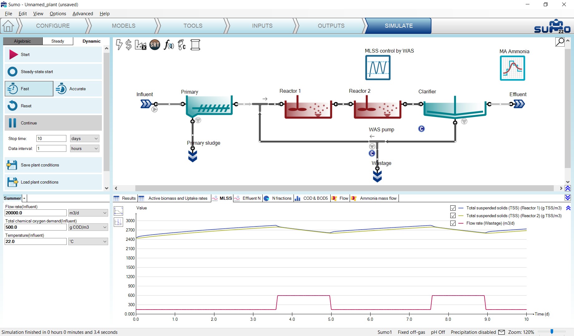
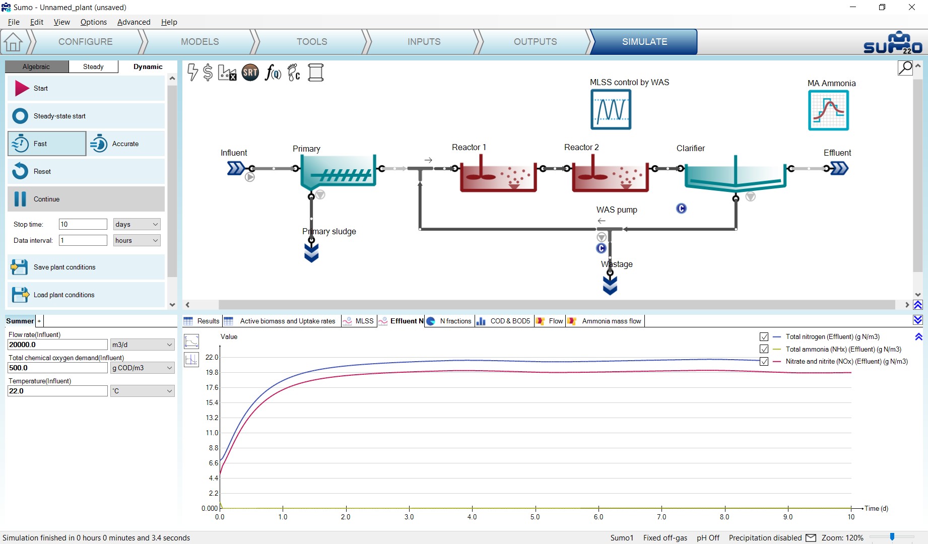
A 10-day MLSS graph gives a good indication whether the system has settled into stable condition and the results are meaningful for typical dry weather summer operation, so let us start by setting the stop time to 10 days with 1-hour data interval and running a dynamic simulation. MLSS and effluent N plots are presented by Figure 3.35 and Figure 3.36, respectively. The effect of the MLSS control strategy can be observed as well.
In the bottom left screen panel rename the Default scenario to Summer (in order to differentiate from an another scenario that will be added later on).
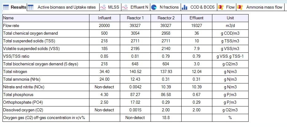
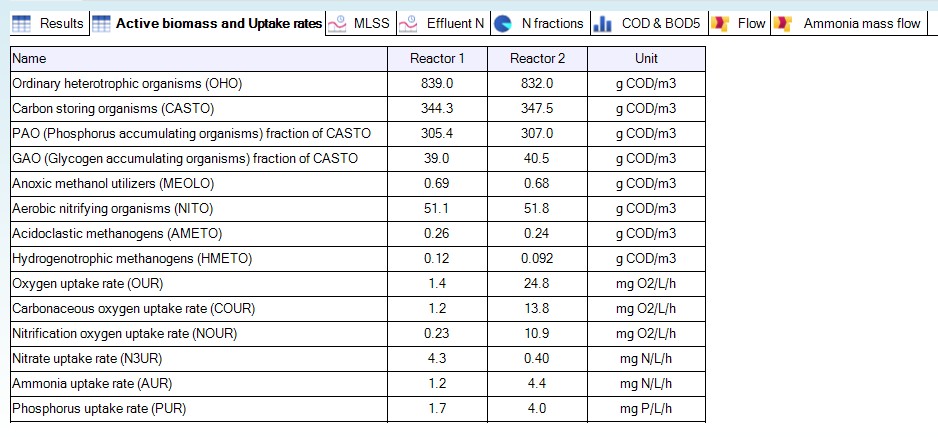
The tabular results are shown in Figure 3.37 and Figure 3.38.
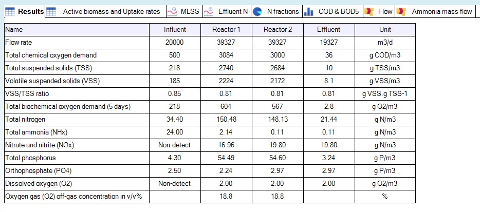
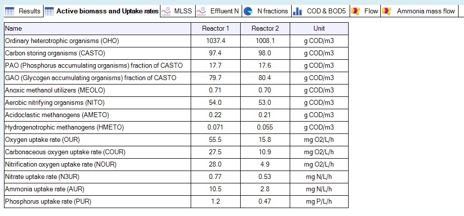
These tables show:
- TSS and VSS profile from the influent through the reactors to the effluent;
- High effluent nitrate and low effluent ammonia (full nitrification);
- DO of 2 mg/L in both reactors (due to input settings);
- Oxygen Uptake Rate (OUR) in the two reactors: higher in the first one, lower in the second, as expected.
This fully aerobic plant does nitrify completely, producing low ammonia and high nitrate concentrations in the effluent. Both reactors are aerated to 2 mg/L DO, which requires energy and comes with costs.
¶ Implementing denitrification
In the system above, the main electron acceptor for biochemical reactions is dissolved oxygen. We can use the abundant nitrate as electron acceptor, and with this process reduce our energy requirement and improve the effluent quality at the same time. For this, we need to reconfigure the plant – in this case simply creating an anoxic zone by switching off the aeration in Reactor 1. (In the actual plant, mixers would need to be installed in the anoxic zone to keep the MLSS in suspension, but in the model, the reactors are always ideally mixed.)
To implement this change, select Inputs on the Task Bar, switch to Constants mode, select Reactor 1 and select the Aeration settings item from the Input parameters (bottom left panel), then change the DO setpoint to zero in the bottom right panel (Figure 3.39).
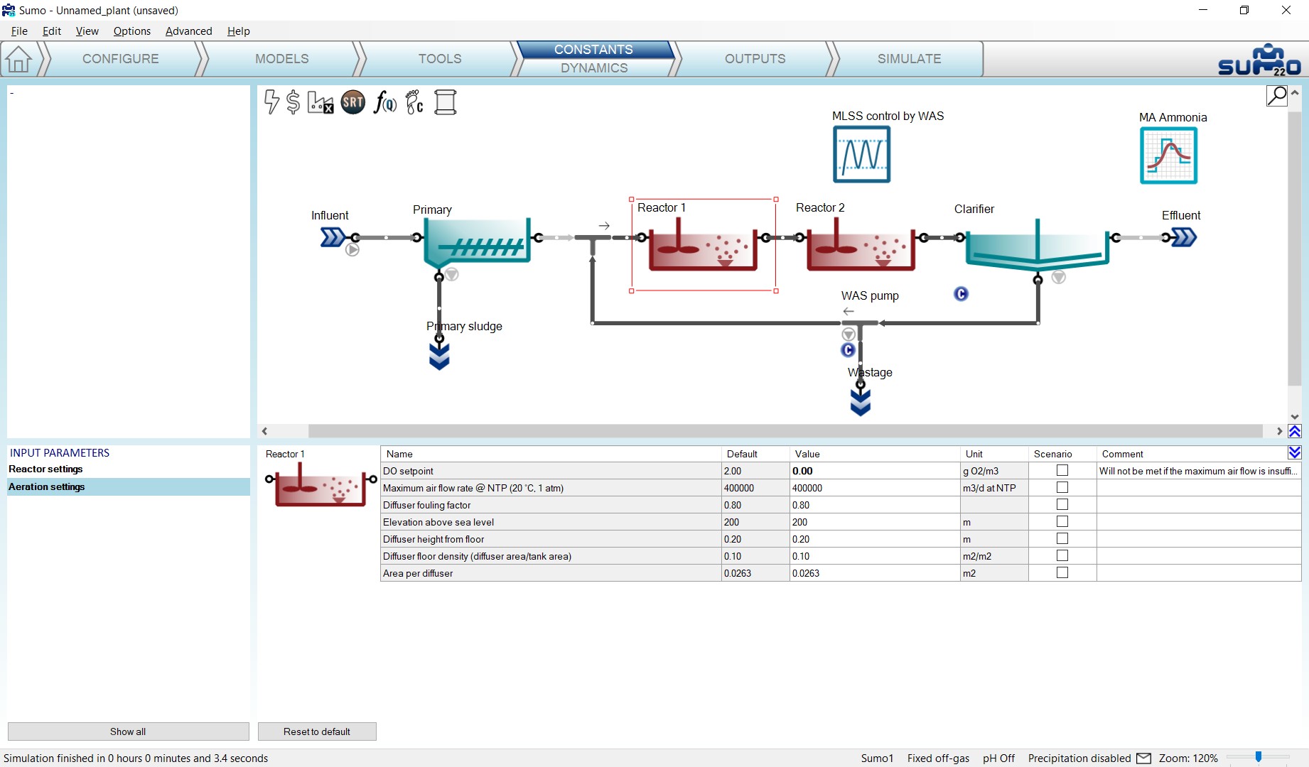
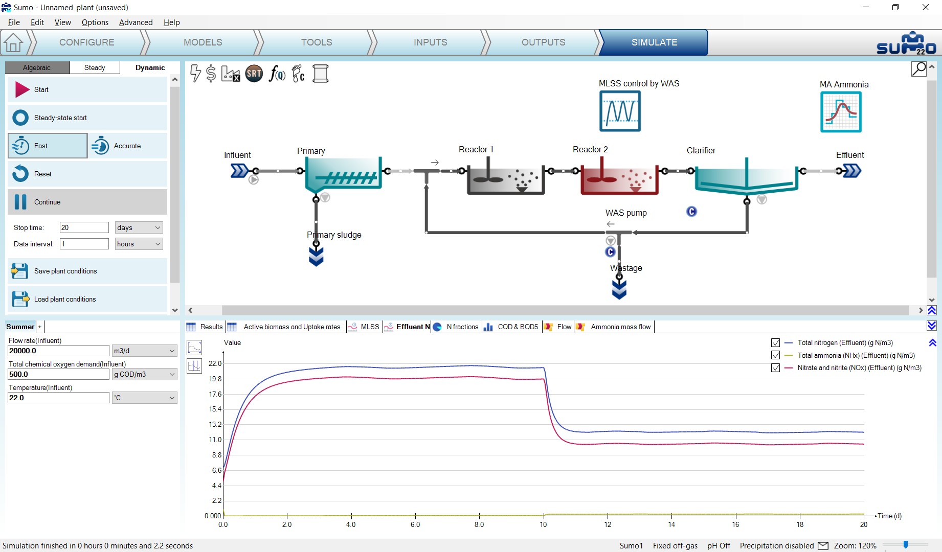
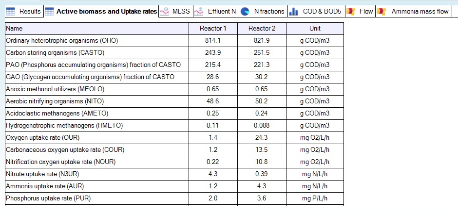
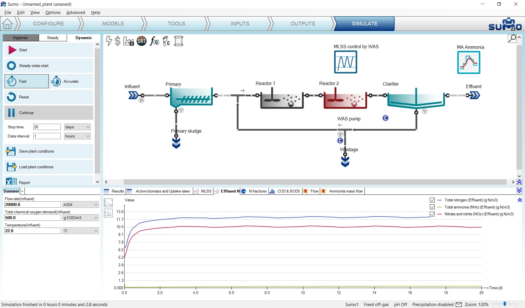
Go back to the Simulate tab, set the Stop time to 20 day and click Continue to go on with the simulation while keeping the results of the previous 10 days in the graphs. Note that the color of the first tank will change to grey: this feature serves for easier visual identification of anoxic/anaerobic reactors. The effluent nitrate will be reduced because it is used up to oxidize organic material in Reactor 1 (the anoxic zone). On the contrary, effluent ammonia increases slightly as nitrification requires aerobic conditions and the aerobic reactor volume was reduced from 10000 m3 to 8000 m3. The effect of the DO setpoint change in the Reactor 1 can be followed in Figure 3.40. The drop in effluent nitrate concentration after 10 days is a due to the Reactor 1 having been turned anoxic. The time frame of the change can be followed as well: within 24 hours the nitrate concentration drops to the lower value.

Besides calculating air flow from a defined input DO, Sumo also offers the possibility to calculate DO levels based on specified input air flow. To select this model option, go back to the Configure tab and select Reactor 1, then in the Dissolved oxygen process unit option, switch from Input to Calculated (Figure 3.43). The calculated DO option will provide a better estimate of expected effluent values. In an aerobic reactor, instead of DO setpoint, the air flow is defined in the Inputs, and the concentration of the DO is calculated based on a mass transfer model. In anoxic (and anaerobic) reactors, with zero airflow specified, only the DO introduced by their input flow is considered.
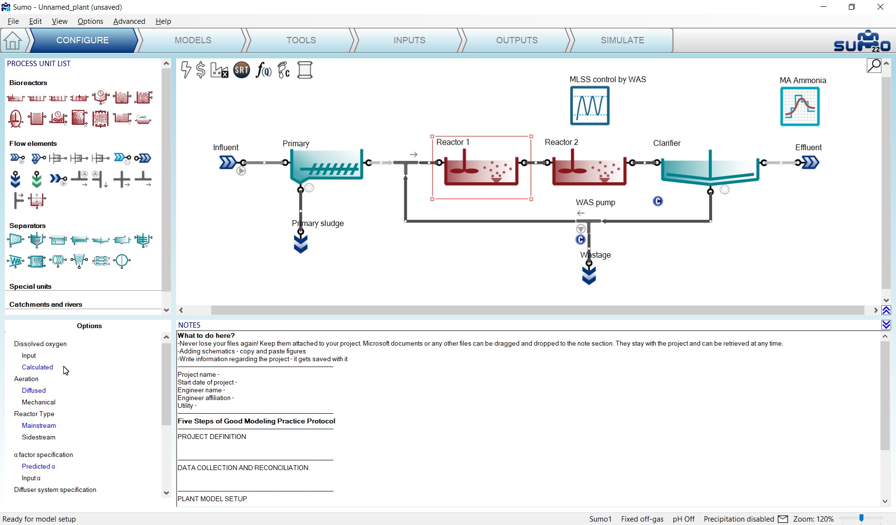
The air flow can be provided on the Inputs tab. Let us change the blower airflow of Reactor 1 to 0 (Figure 3.44):

After clicking on Reset, then running a 20-day simulation, you can compare the results of the plant operating with input DO (Figure 3.40, Figure 3.41 and Figure 3.42) and the plant operating with calculated DO (Figure 3.45, Figure 3.46 and Figure 3.47):
¶ Subjecting the plant to dynamics
Plants are usually subjected to diurnal variation and we might be interested not only in the average, but the peak effluent concentrations as well (e.g. in certain jurisdictions the effluent limits are based on grab samples never to exceed, daily maximum, etc.). This requires a dynamic simulation to investigate potential peaks during the day.
Select the Inputs tab, and the Influent process unit, where we will provide diurnal flow variation. In Constants mode, the Influent tool is available for Sumo models as an Excel file, containing typical fractions and diurnal variations with different plant sizes. Click on the button (located in the bottom right screen panel) to open this tool and copy the “medium plant” table from the Diurnal flow sheet to the clipboard (Figure 3.48):
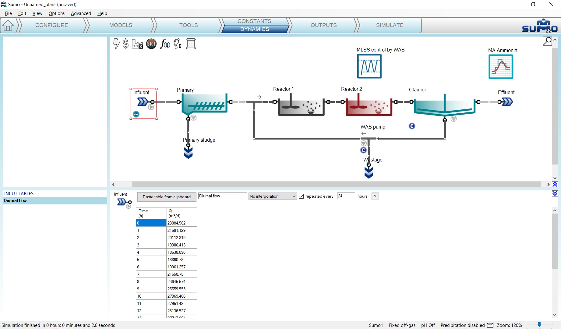
Now switch to Dynamics mode in Sumo and paste your table by clicking on the Paste table form clipboard button (after this, you can close the Influent tool Excel file). On the drawing board, a small sign will appear below the Influent, showing that dynamic parameter input is used. These tables can be disabled/enabled or deleted by right-clicking on the name in the bottom left screen panel. Note that for a certain variable/parameter, only one dynamic table can remain enabled (Sumo will give you a warning if more than one tables are enabled for the same subject). The names of disabled tables (which are editable in the bottom right screen panel) will show up in grey, and in case all dynamic input tables are disabled, the sign beside the process unit will also turn to grey (indicating that there are dynamic inputs available, but not used). Linear interpolation and cycle repeat can also be set for dynamic input tables. Rename the newly inserted dynamic input table in the example to “Diurnal flow”, check the box to repeat the contents of the table and provide the repeat frequency as 24 hours in this example, as depicted on Figure 3.49.
If you can provide data from measurement, your input data (flow variation in this case) should be in Excel, in the following format: the header should be “Time” (“time” is also accepted) and the selected variable name as it is used by Sumo, in this case “Q” (denoting flow), with the respective units (“h” and “m3/d”) in the second row, as illustrated by Table 3.6.
Table 3.6 – Dynamic input of influent flow pattern
|
time |
Q |
|---|---|
|
h |
m3/d |
|
0.0 |
23084.502 |
|
1.0 |
21581.129 |
|
2.0 |
20112.819 |
|
3.0 |
19006.413 |
|
4.0 |
18538.096 |
|
5.0 |
18860.780 |
|
6.0 |
19961.257 |
|
7.0 |
21658.750 |
|
8.0 |
23645.574 |
|
9.0 |
25559.553 |
|
10.0 |
27069.466 |
|
11.0 |
27951.420 |
|
12.0 |
28136.527 |
|
13.0 |
27717.954 |
|
14.0 |
26916.230 |
|
15.0 |
26012.768 |
|
16.0 |
25269.925 |
|
17.0 |
24859.318 |
|
18.0 |
24817.715 |
|
19.0 |
25042.167 |
|
20.0 |
25325.377 |
|
21.0 |
25421.266 |
|
22.0 |
25122.513 |
|
23.0 |
24328.482 |
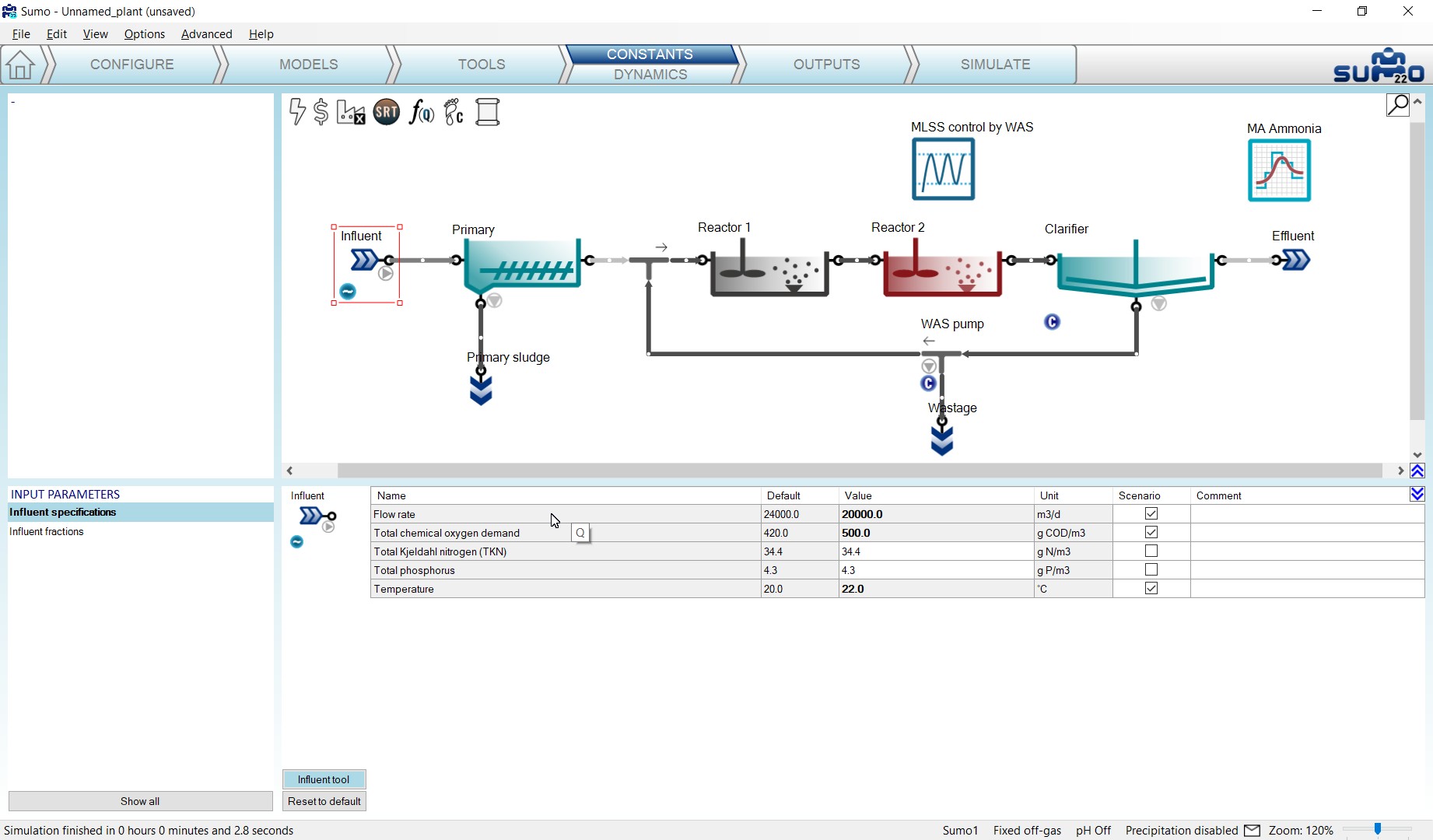
To find out what is the internal identifier for a certain variable (or model parameter), you can just hover the mouse above the name of the specific item in the parameter tables of Inputs – Constants (or in the case of model parameters, the Models), and a popup will show you the cryptic name of your input variable that has to be used in the dynamic table (see Figure 3.50). For your comfort, right-clicking here offers an option to copy this symbol directly to the clipboard (and the same goes for units), from where you can paste it into your table.
Having set up the diurnal flow, go to the Simulate tab and start a new dynamic simulation of 5 days duration: In this case, the result of the last simulation will be used as initial values. The variation in loading should have an effect on effluent quality, as shown by Figure 3.51.
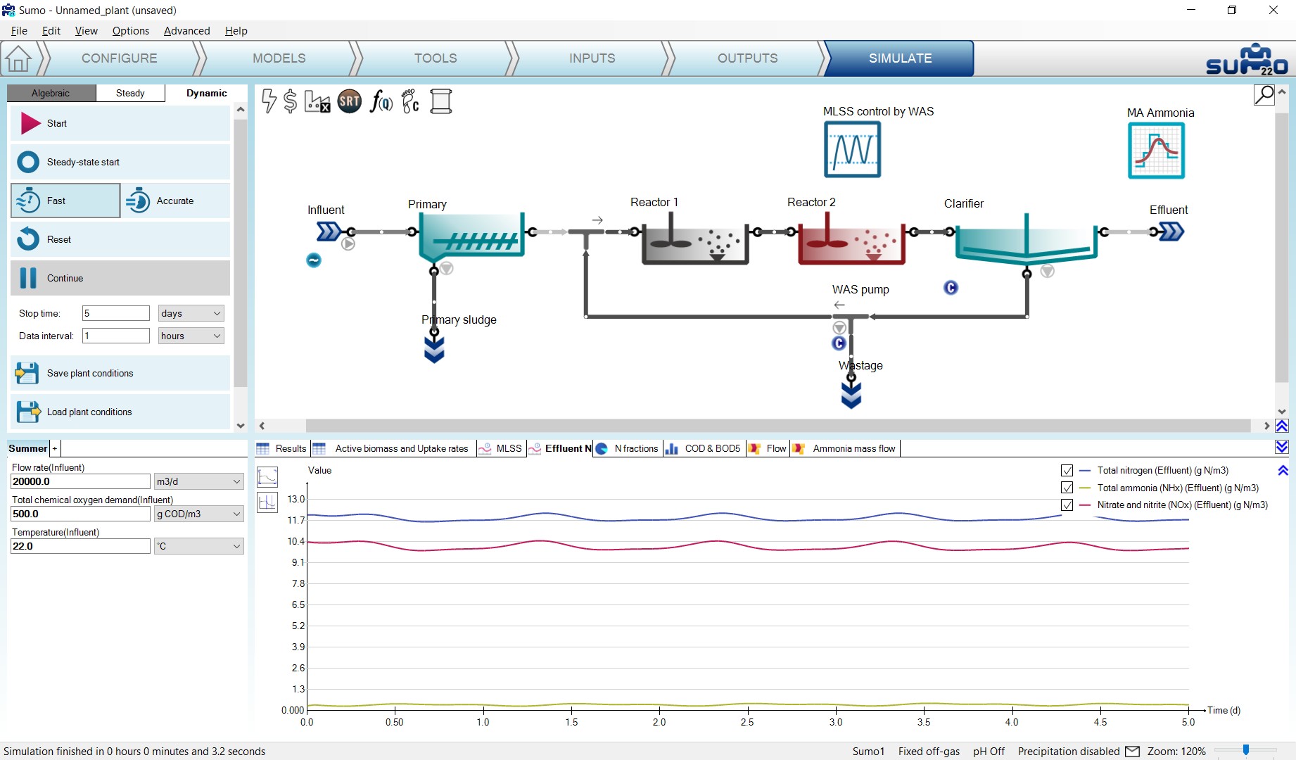
We can observe higher ammonia concentrations during the high loaded periods, and lower nitrate concentrations, due to lower nitrification and the abundance of organic substrate for denitrification.
We can of course always turn on our aerators in the first reactor (not so easy in an actual plant) by going to the Inputs tab, selecting Reactor 1 and changing the air flow to 150000 Nm3/d. In the Simulate tab, we can extend the length of the run for 10 days and hit Continue.
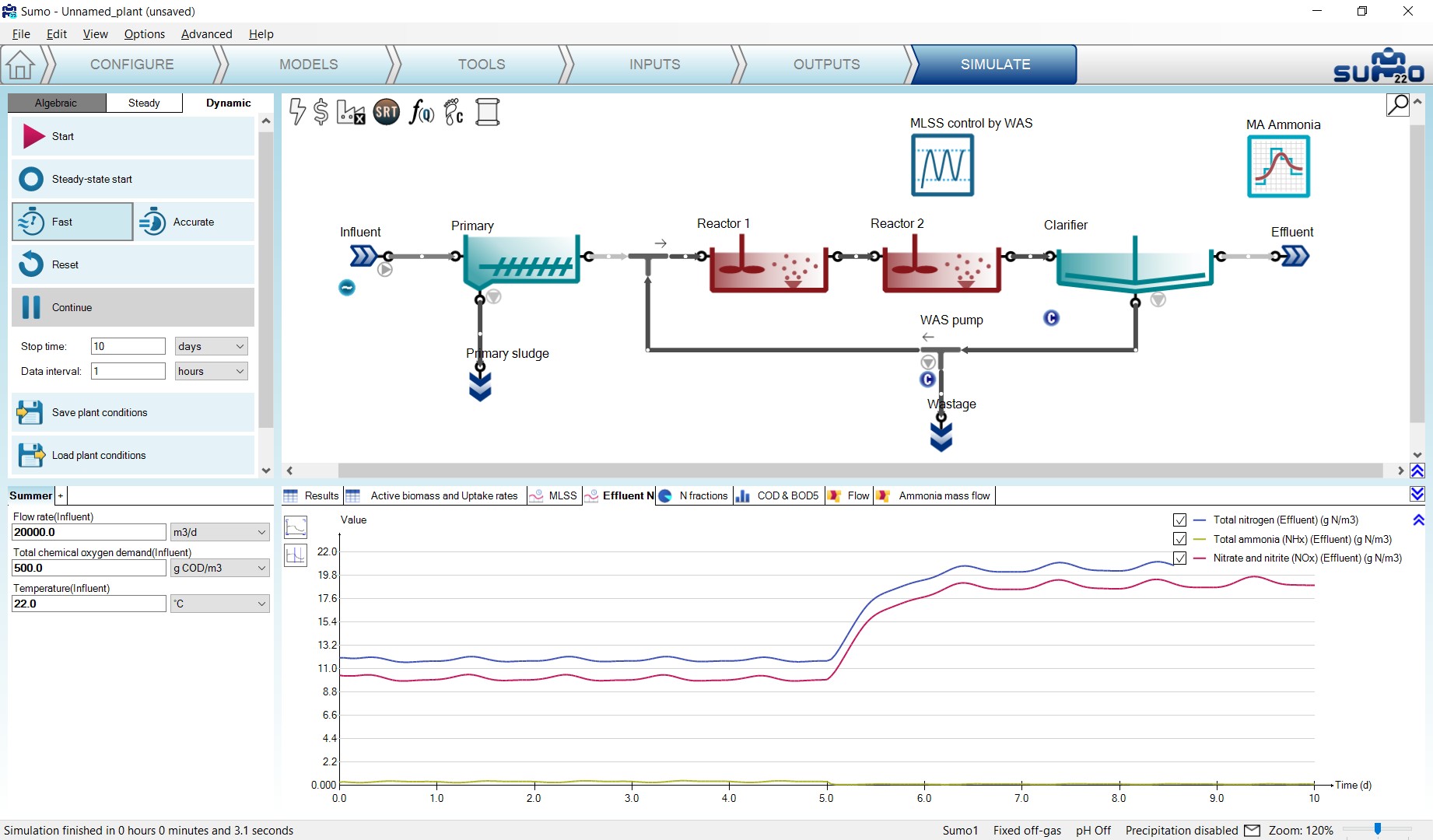
Nitrate concentration will increase, and the ammonia peaks will get much reduced from day 5, when the aerators were turned back on. After this exercise, reset the air flow in Reactor 1 to 0 Nm3/d and run a 10 d simulation to get back to denitrifying plant.
¶ Model parameter dynamic input
Model parameters and plantwide parameters can be added as dynamic inputs as well – in these cases, the plantwide (factory) icon should be selected on the drawing board in the Inputs – Dynamics tab, and extended descriptions of the model parameters are to be used in the dynamic input tables, as described below.
The incode name of model parameters can be found as popup by hovering the mouse over the desired parameter on the Models tab. See the example of Maximum specific growth rate of the NITOs (nitrifier organisms) on Figure 3.53: µNITO is the name of the parameter in the active model, which is the Sumo1 model in this tutorial.
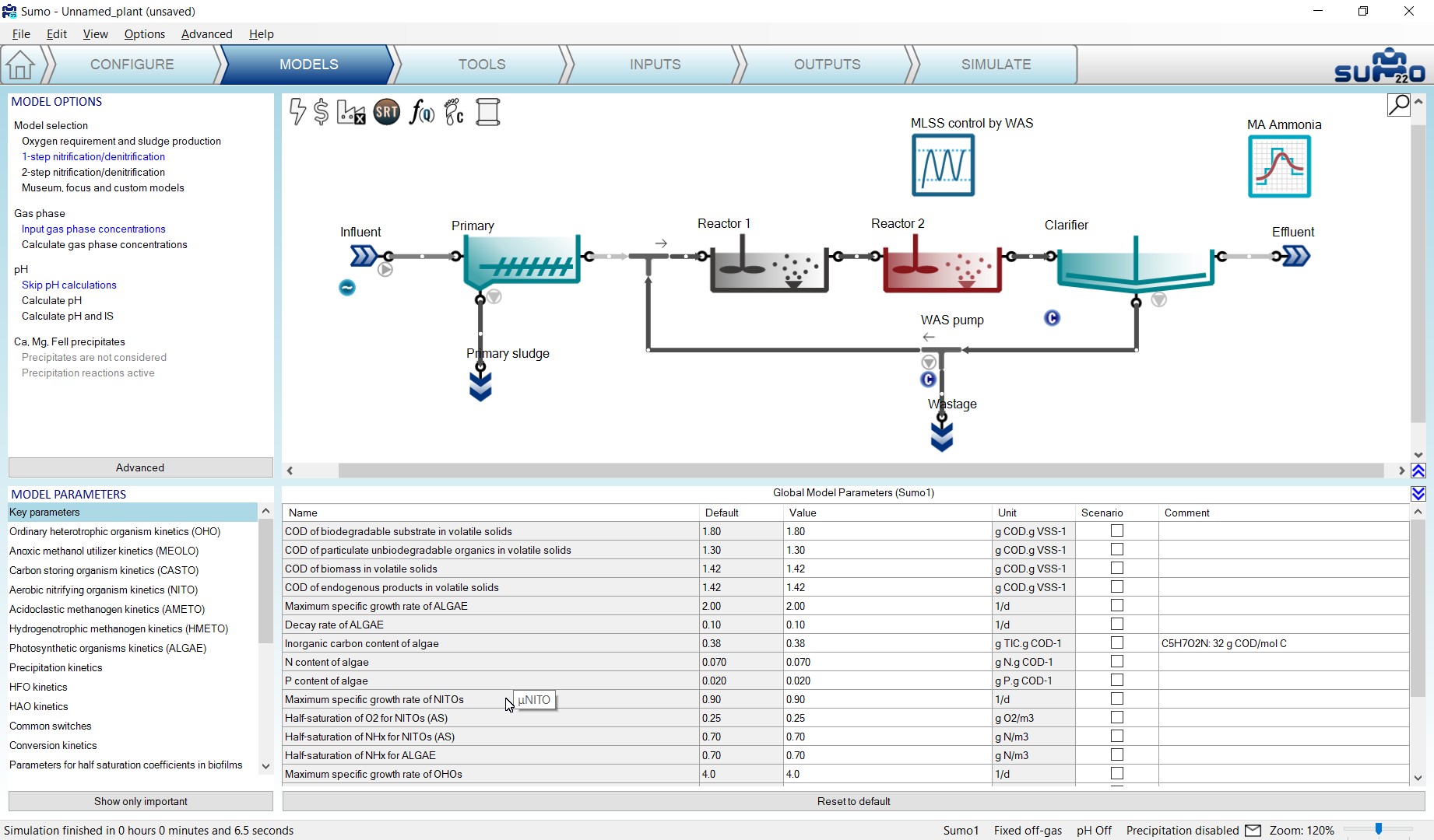
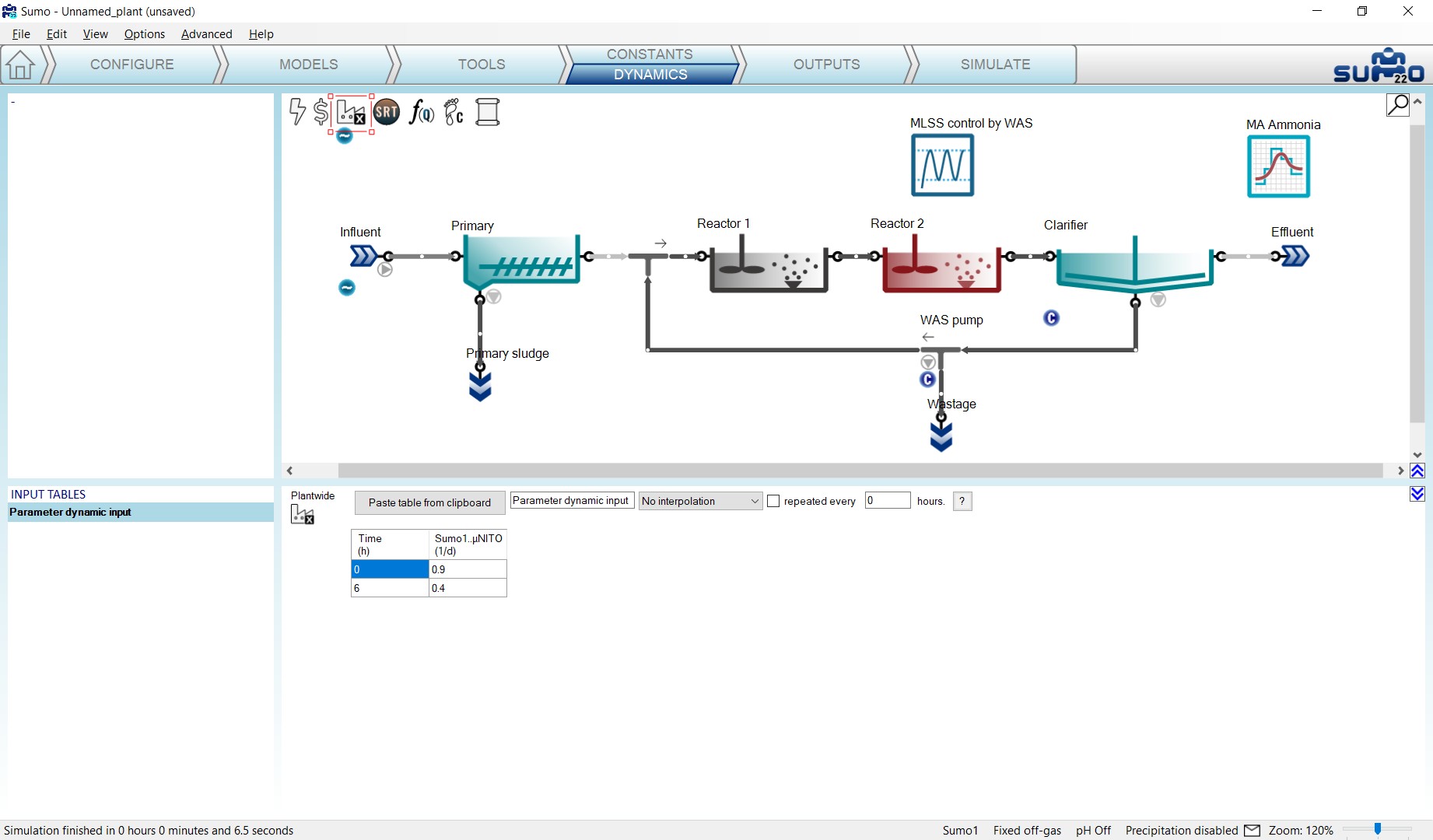
The model name of the parameter is the compound of the model name and the parameter name, separated by two dots. So in our example, Sumo1..µNITO will be the correct model parameter name to be used in the dynamic input table (Table 3.7).
Table 3.7 – Model parameter dynamic input table
|
time |
Sumo1..µNITO |
|
h |
1/d |
|
0.0 |
0.9 |
|
6.0 |
0.4 |
Inserting the dynamic input table is done the same way as it was done in the diurnal flow – just copy the prepared table from Excel and paste using the button in the Inputs – Dynamics tab (remember that the factory icon shall be selected for showing this functionality). The presence of the dynamic global model parameter input will be indicated by a blue circle with a wave inside on the drawing board, below the factory icon (see Figure 3.54).
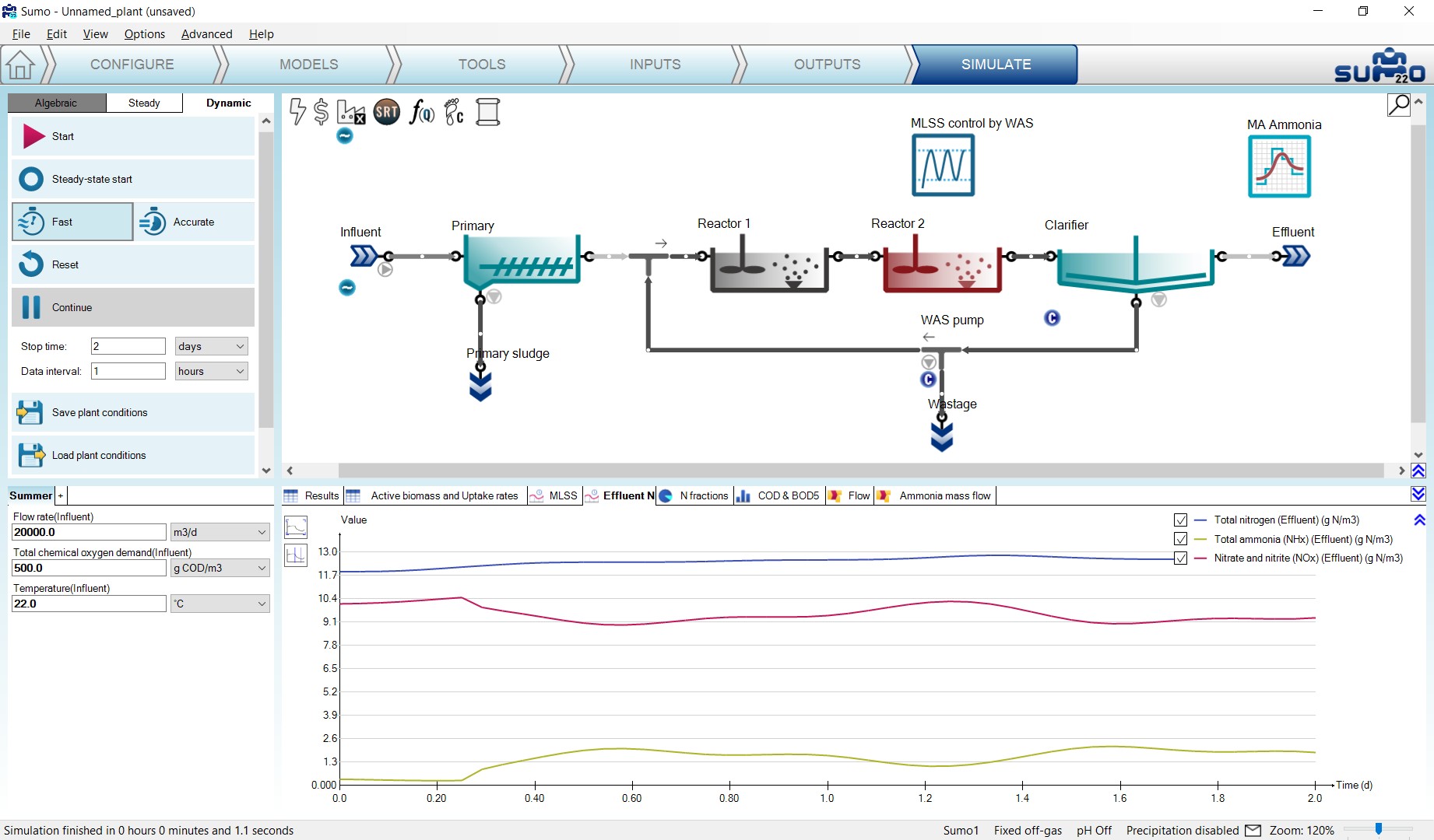
Now let us go to the Simulate tab and start a 2-day simulation with an hourly data interval. The decrease in nitrifier maximum growth rate (caused by i.e. a toxic substance in the influent) should have an effect on effluent quality as shown in Figure 3.55: we can observe higher ammonia concentrations after the decrease in the NITO growth rate.
During the following exercises, we will not use the dynamic input for model parameters any more. In the bottom left screen panel of the Inputs/Dynamics tab, right click on the name of this table and choose Delete table to remove the table. Alternatively, you can just use the Disable table option as well, in order to keep the table but not to use it during the subsequent simulation. Let us try this option for switching off the diurnal flow (the indicator below the Influent icon will turn to light grey).
¶ Adding measured data to the charts
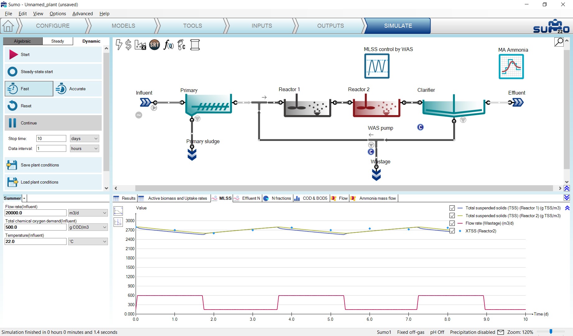
Plants do collect information and one important task in process simulation is to compare measured data with simulation results (and potentially using the information to calibrate the model). Let us assume that this plant has MLSS grab samples once a day in Reactor 2 (TSS Reactor 2). The collected data is shown in Table 3.8 below.
Table 3.8 – Measured TSS data for the example plant
|
Time |
XTSS (Reactor2) |
|
d |
g/m3 |
|
0 |
2800 |
|
1 |
2700 |
|
2 |
2600 |
|
3 |
2700 |
|
4 |
2780 |
|
5 |
2700 |
|
6 |
2750 |
|
7 |
2725 |
|
8 |
2775 |
|
9 |
2600 |
|
10 |
2750 |
Copy this table into an Excel sheet (e.g. named Plant Data.xlsx) and rename the sheet “Measured TSS” (Actual names are irrelevant and flexible).
Switch Sumo to Simulate mode, click on Reset, then run a 10-day simulation to let the system settle into stable condition. Then run another 10-day simulation for evaluating the MLSS trend due to the deadband controller.
Switch Sumo to Outputs mode, right click on the MLSS timechart tab and select Import data. The data import is carried out the same way as the dynamic input table: simply paste from the clipboard (Figure 3.56).
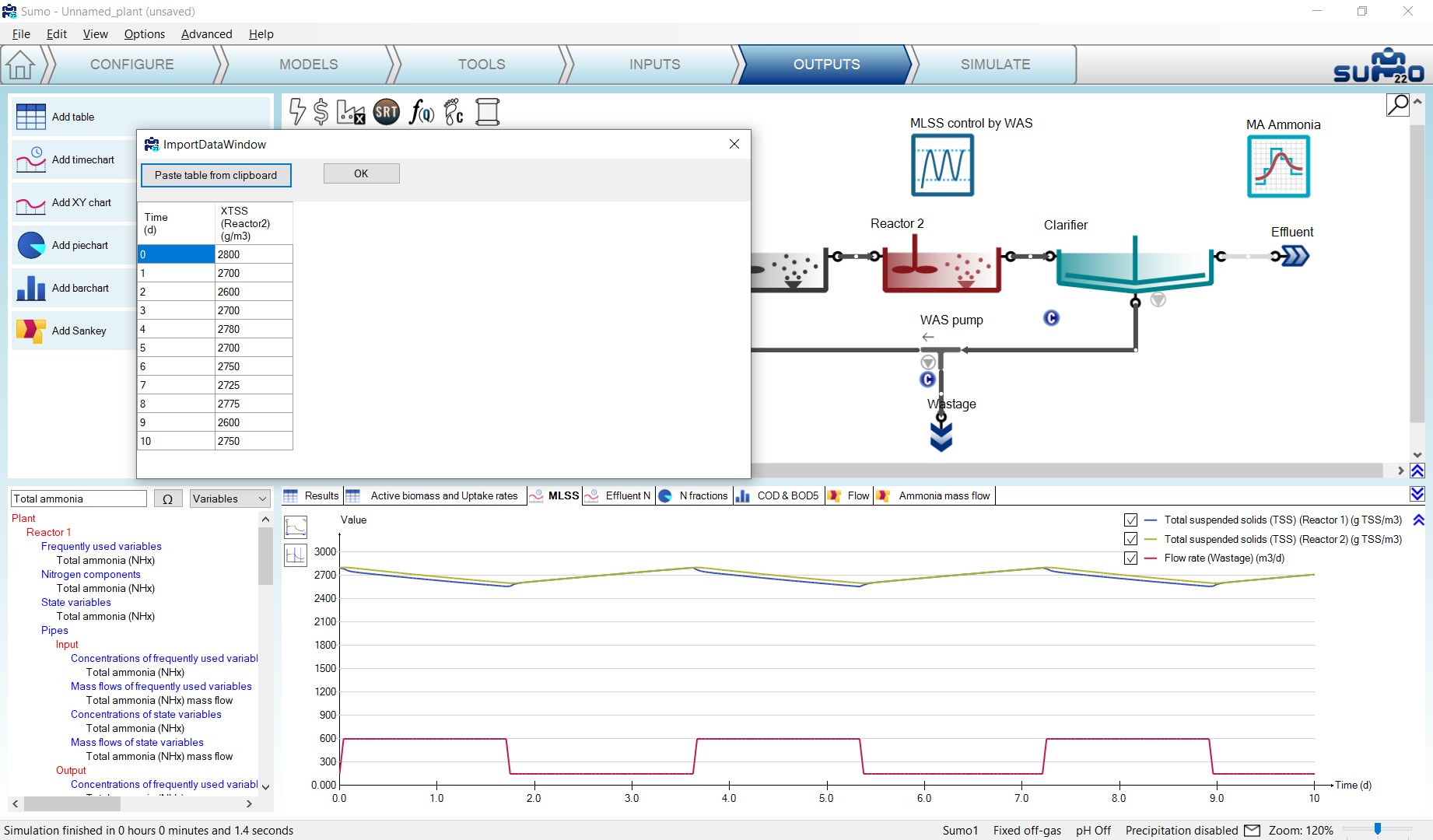
Pressing OK the data is plotted along the simulation results (Figure 3.57):
The project can be saved any time during the configuration and project development using the File menu and reloaded at a later point in time to continue the work.
Many other operational scenarios can be simulated with Sumo, including more complex reactor configurations and more elaborate operational scenarios. Please see Examples under the Help menu and for further description check out the Examples chapter of this manual.
¶ Scenarios
By default, the simulation is using the input parameters defined in Inputs, such as the influent flow rate, the influent Total Chemical Oxygen Demand and the influent temperature, which we have also selected for scenario analysis at an earlier stage. On the bottom left screen panel of the Simulate tab, further scenarios can be defined by clicking on the Add Scenario (+) tab. Add a new scenario, rename it to Winter and set 14°C, 26000 m3/d flow rate and 460 mg O2/l COD as input parameters instead of the default parameter set provided in the Summer tab. (Figure 3.58). With this simple setup the simulation will now use (as long as the Winter tab is active) 14°C as influent wastewater temperature, modified influent flow and COD composition and the results can be compared.
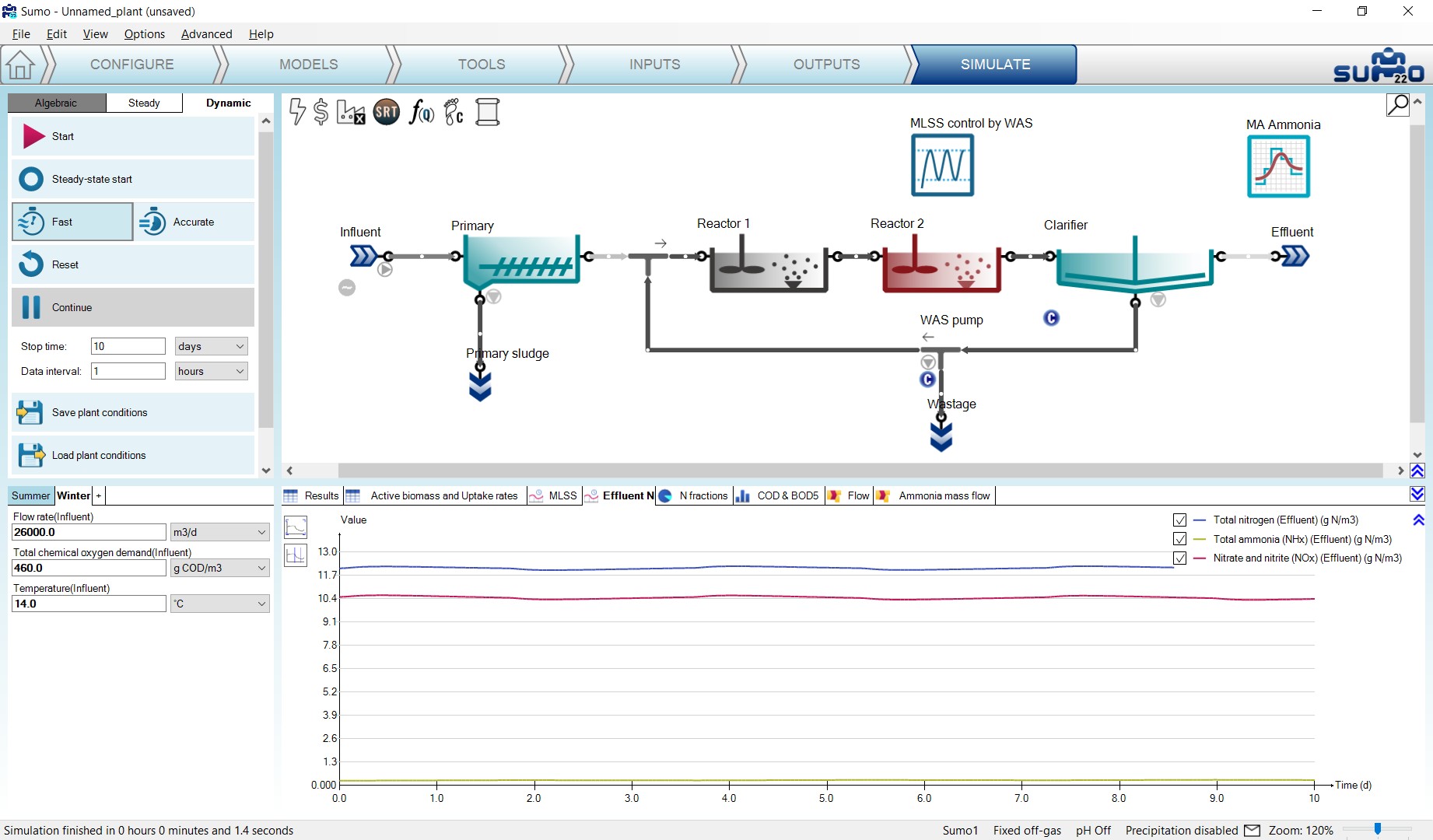
After clicking on Reset and running two consecutive 10-day dynamic simulations (in order to get the system to a characteristic winter operation), activate the Summer scenario by clicking on its tab, modify the simulation stop time to 20 day and hit Continue. The change due to new influent conditions can be seen quickly (Figure 3.59):
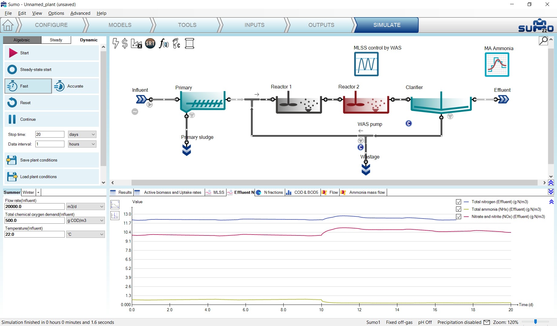
If you want to add further parameters, just go back to the Inputs tab and select the desired parameters of the desired process unit. Model parameters can be selected as well for scenario analysis and the Models tab.
¶ Adding popups
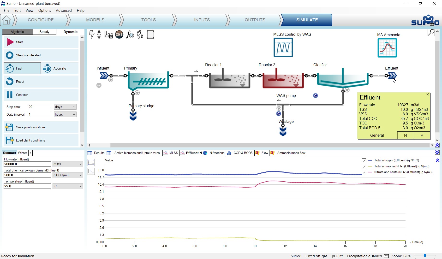
If you hover above any process unit on the Simulate tab with the mouse and leave it there for a second, a yellow popup will appear with a summary table of the most important variables related to that process unit type (Figure 3.60). Moving the mouse elsewhere will make the popup disappear soon after. However, if you grab it with the mouse while it is active and place it somewhere in the layout, it will remain there as a sticky note as long as you don't close it with the X in the top right corner. Most popups will have a few tabs in the bottom which you can toggle when the popup is active, in order to reveal more information.
¶ Adding pipe info tables
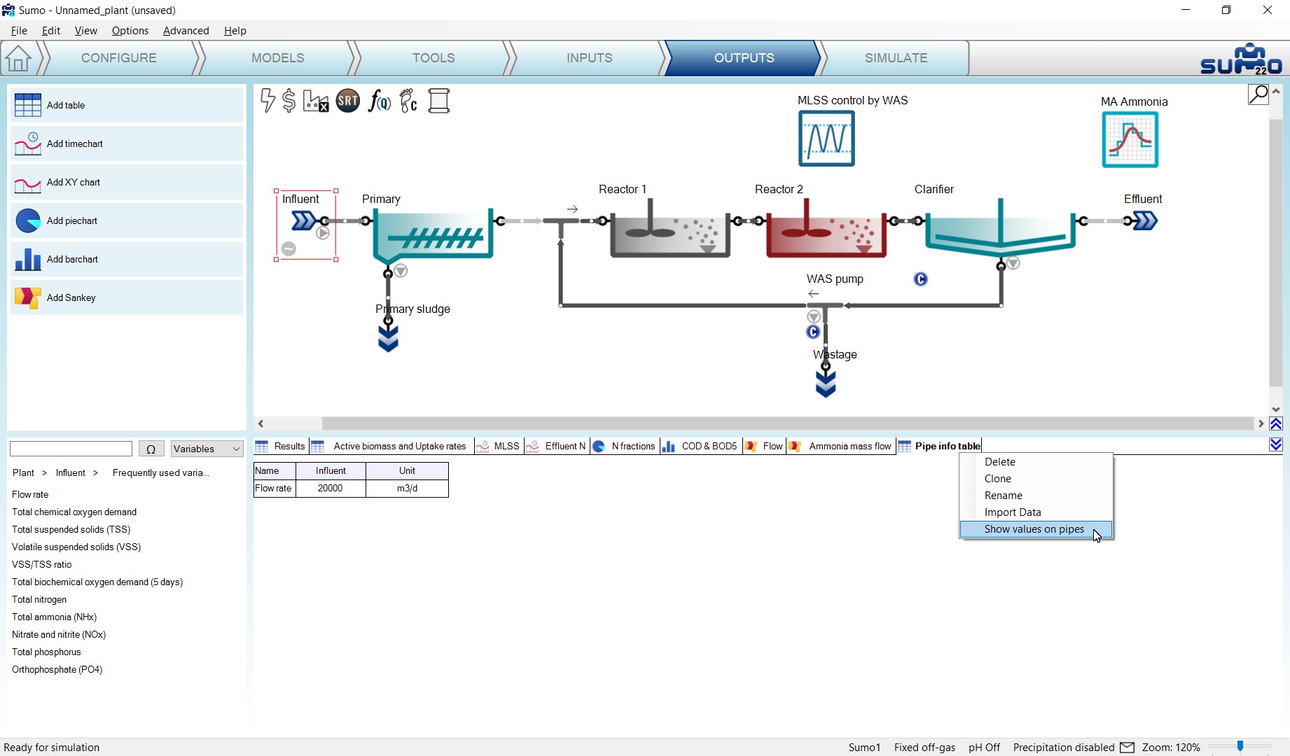
Data from any table can be set to be shown on the pipes of the layout. For an excercise, let's go back to the Outputs tab and add a table with the Flow rate of the Influent process unit (can be found under Frequently used variables). Rename the table to Pipe info table and right click on the name tab, then click the Show values on pipes option (Figure 3.61).
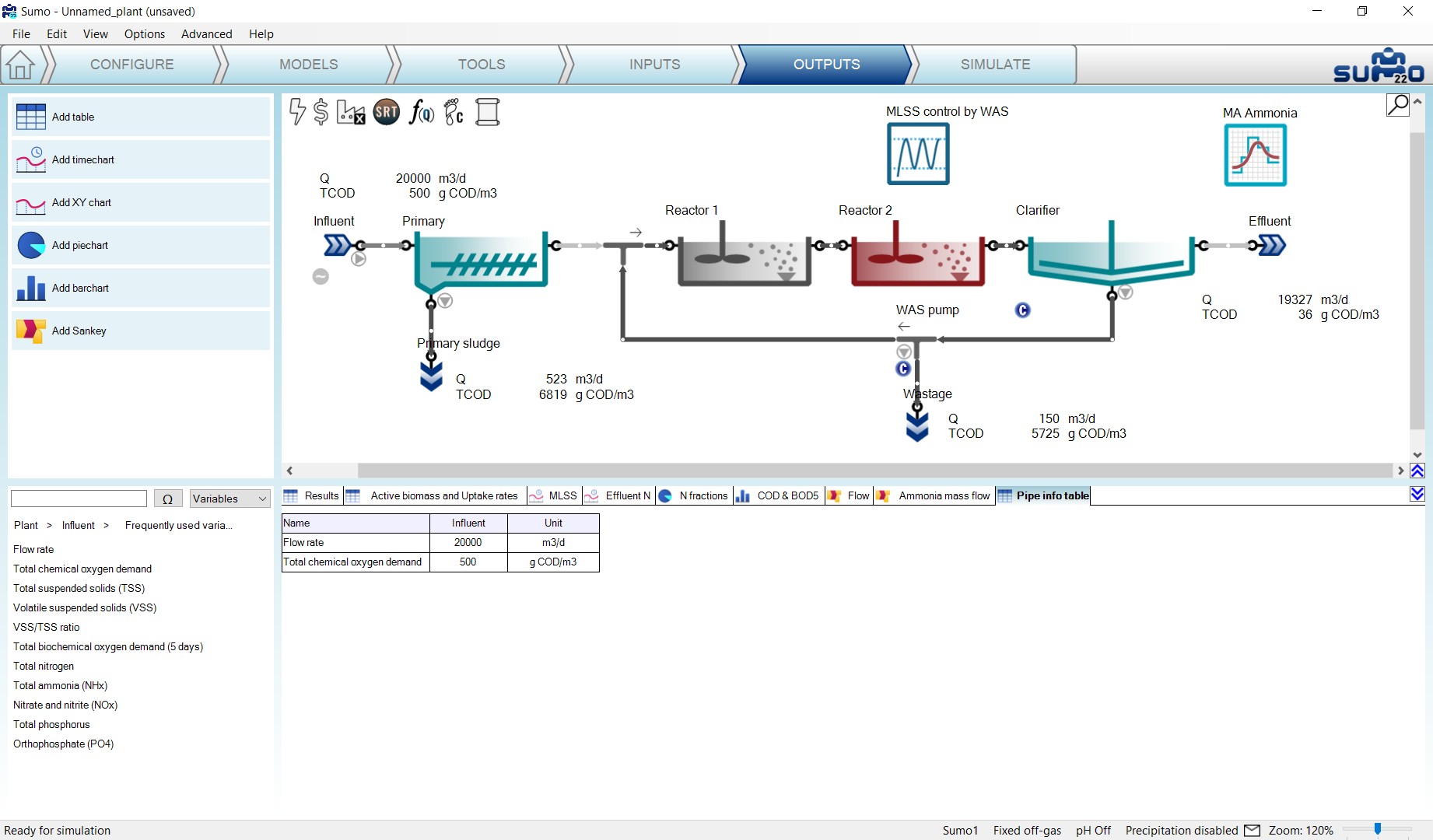
This will add a transparent popup nearby ALL pipes of the configuration. In most cases you will only need a handful of them, so you can remove the unnecessary ones by clicking the X in the top right corner of the unwanted popups. For the excercise, keep only the ones belonging to Influent, Effluent, Primary sludge and Wastage. By dragging and dropping, you can reposition the pipe info popups for better readability. If you add further variables to the source table, you will see that they will be shown on the popups as well (Figure 3.62). Along the same line, removing variables from the source table will remove them from the pipe info, too.
¶ Writing a report
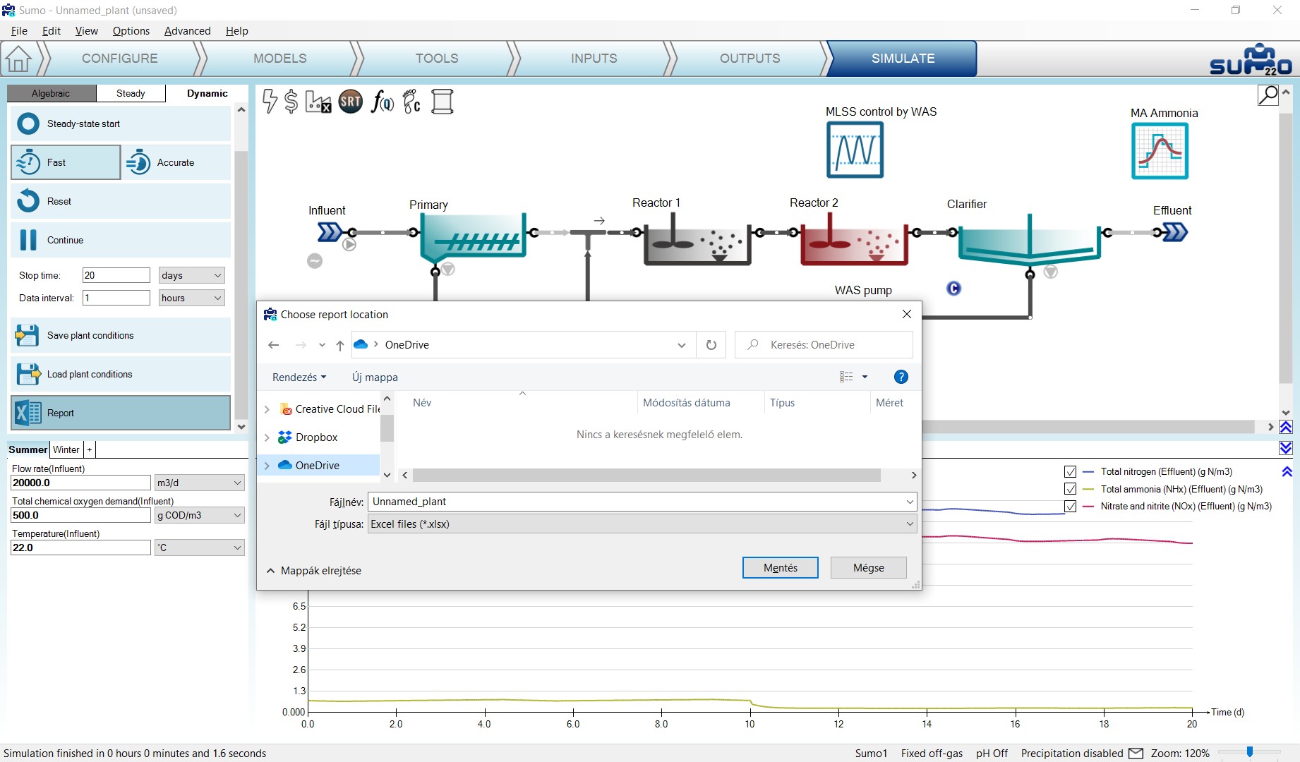
On the Control panel of the Simulate tab, a Report button is available. When clicked, results will be written to an Excel file, available for further processing. The resulting Excel file is named the same as the sumo project file by default (Figure 3.63). This function creates an Excel file with the following sheets:
- Project overview: contains the configuration layout and basic project information
- Notes: the contents of the Notes screen panel from the Configuration tab
- Modified parameters: values of all parameters in the project that were changed from default
- Scenarios: values of parameters in the scenarios
- Simulation results: all results of the output tabs get saved to separate sheets, including data tables for the diagrams
- Model: contains all parameter values for the used model (in this example: Sumo1)
- Plantwide calculations: Plantwide, Energy center, Cost center, SRT and Flow dependence settings are saved on separate sheets
- Process Units: all settings and PU parameters are displayed on separate sheets for each unit, including pipes.
- Controllers: all settings and parameters of the controllers employed in the project (if any).
¶ Controllers
Controllers are used to set operational parameters based on measured values during the operation of the plant. In Sumo, the controlled values are calculated variables from the simulation. The on-off controller has no controlled variable. The manipulated parameters are input values for the controlled process unit. For example, this way the reactor MLSS can be automatically controlled by manipulating the wastage sludge flow. Another example is setting the air flow into the aerated reactor to maintain a certain dissolved oxygen level.
There are 6 different type of controllers implemented in Sumo, which can be added on the Tools tab (Figure 4.1):

Clicking the Controllers button on the Tools tab will open this dropdown list of controllers, where you can pick the desired one and configure the control variable (CV) and the manipulated variable (MV) which is a parameter in the model; while on the Inputs tab you can fine tune the controller settings. In this chapter, the setup possibilities will be presented for each available controller one by one, based on the example project built in the previous chapter (How to use Sumo for simulations).
¶ Continuous P controller
The Continuous P controller is a model controller that continuously sets (integrates) the input parameter (Manipulated variable) of the desired unit to meet the control variable value setpoint (as opposed to discrete controllers).
Add this controller to the layout from the Tools and configure it as follows. First drag and drop the manipulated process unit (Reactor 2) to the left side of the equation in the bottom right screen panel and the controlled unit (Effluent) to the right side of the equation. On the bottom left screen panel, you can now select the control variable and the manipulated variable in the respective units. In this example, we will manipulate the requested DO setpoint to maintain the desired ammonium concentration in the effluent. Rename the unit (using F2 or right click) to “Ammonia control” (Figure 4.2).
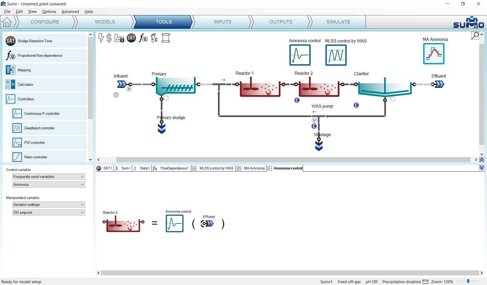
Proceed to the Inputs tab and select the newly added controller. Once the project compiled, in the Controller parameters table, enter the following settings:
- Controlled variable setpoint to 0.5 g N/m3 (target effluent ammonia concentration);
- the Maximum of the manipulated variable value to 3 g O2/m3;
- the Controller direction to -1, because it is an inverse controller (to decrease the ammonia concentration the DO setpoint has to be increased).
At the Controller initialization table, set the Initial value of manipulated variable to 2 g O2/m3 (Input DO setpoint in Reactor 2). Leave the other parameters default (Figure 4.3).

To follow the effect of the controller, you can add the setpoint to the Effluent N timechart on the Outputs tab: select the Ammonia control controller and from the bottom left screen panel, go to Parameters > Controller parameters menu and add Controlled variable setpoint to the timechart. (Figure 4.4).
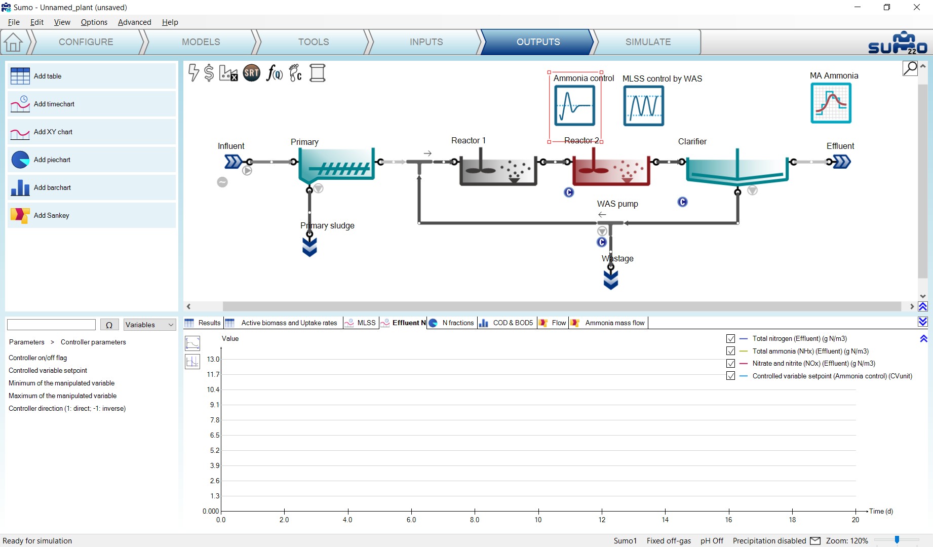
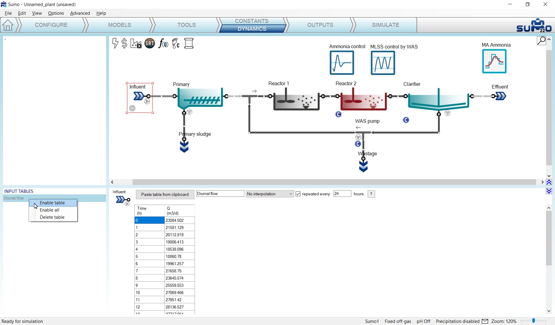
Before starting the simulation, go to the Inputs/Dynamics tab and enable the Diurnal flow dynamic input table of the Influent to have changes in the ammonia load (see Figure 4.5).
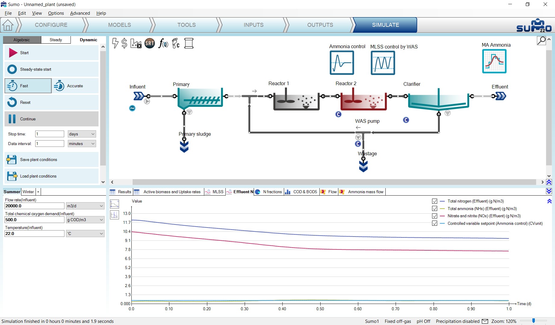
Finally go to the Simulate tab, set the Stop time to 1 day and the Data interval to 1 minute (to see finer details of the operation of the controller) and run the simulation. During the calculation, you can follow the change of the effluent ammonium along with nitrate and nitrite on the previously extended chart (Figure 4.6).
To modify the setpoint of the controller, go to the Inputs tab, select the Ammonia control controller and modify the setpoint to 1.0 g/m3 (effluent ammonia concentration). On the Simulate tab increase the Stop time for 2 days and continue the simulation (Figure 4.7).
Note: Keep in mind that the effluent fluctuation is caused by the influent diurnal flow and the MLSS deadband controller, which are independent of the continuous P controller.
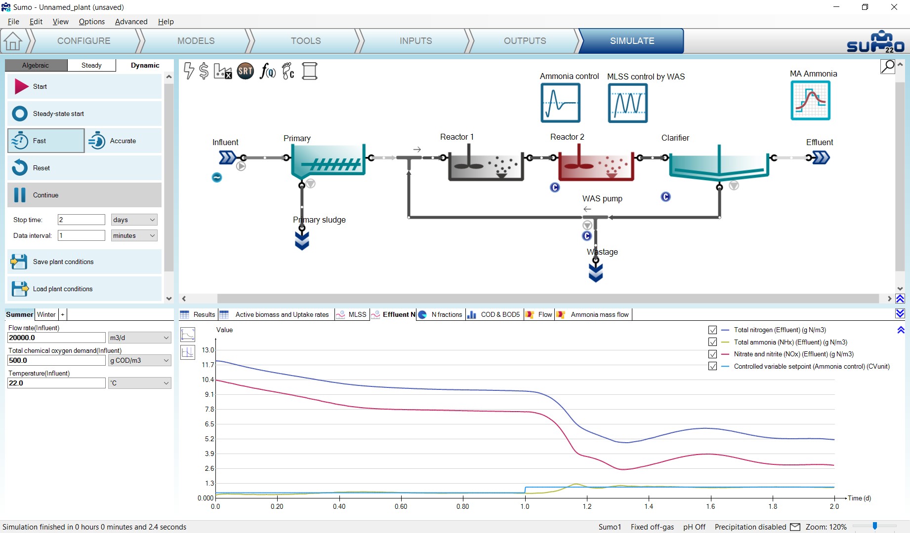
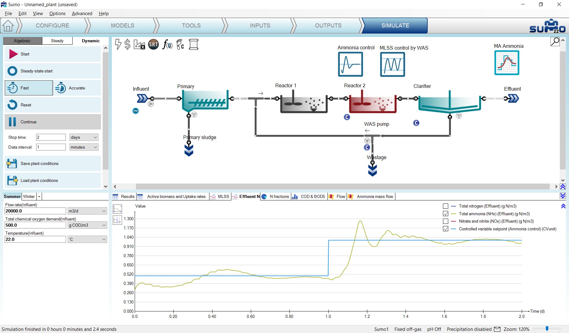
The Total nitrogen and the Nitrate and nitrite (NOx) curves can be unchecked in the graph legend, thus the smooth changes in the effluent caused by the controller DO setpoint modification can be seen in detail. (Figure 4.8)
¶ Deadband controller
In an earlier chapter we added a Deadband controller to manage the MLSS in the reactors.
¶ PID controller
The PID controller is using a discrete time step to set the input parameter (manipulated variable) of the desired unit to meet the controlled variable setpoint.
To demonstrate the capabilities of this controller, let us set Reactor 2 of the example project to use the Calculated option for Dissolved oxygen (Configure tab). Then add the controller and configure on the Tools tab as follows. First drag and drop the manipulated unit (Reactor 2) to the left side of the equation in the bottom right screen panel and the control unit (also Reactor 2) to the right side of the equation. In the bottom left screen panel, you can now select the control variable and the manipulated variable of the selected unit. In this example, we are going to control the requested air flow rate to maintain the desired dissolved oxygen concentration. Rename the controller unit (using F2 or right click) to “DO control by Air flow” – this will rename the tab as well (see Figure 4.9).
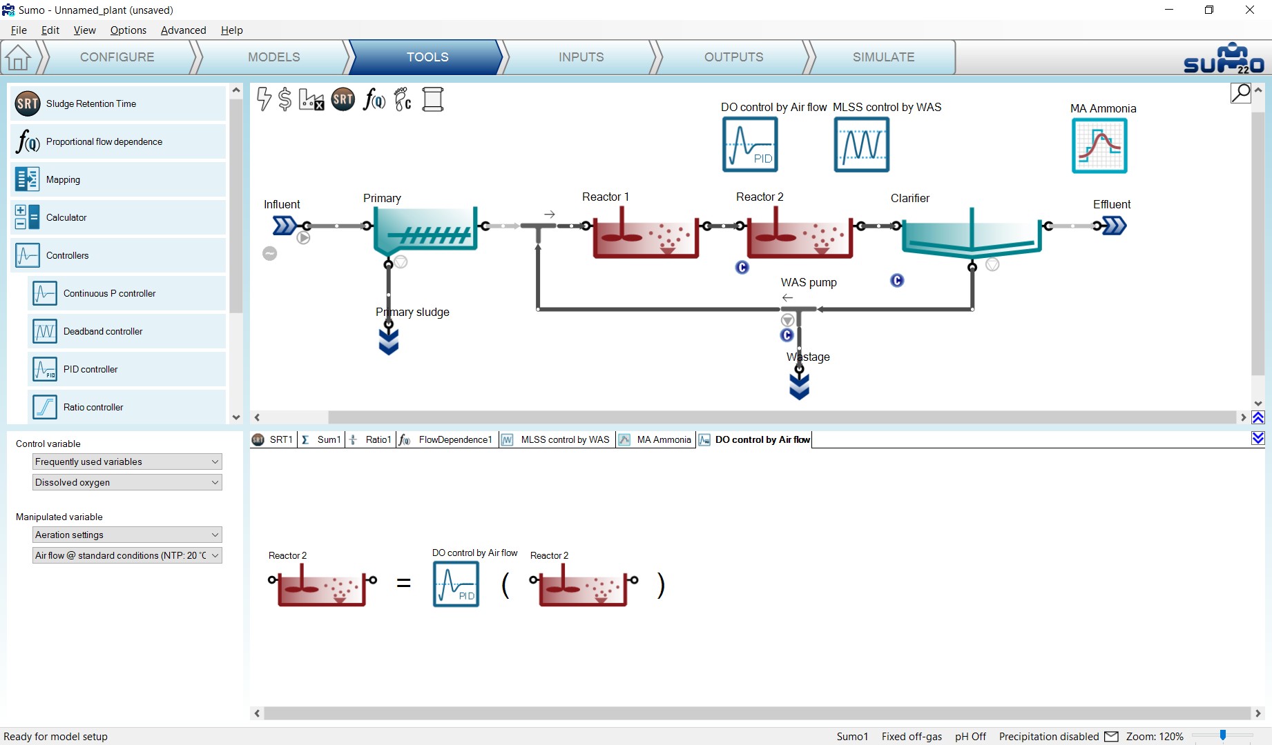
On the Inputs tab, select the newly added DO control by Air flow controller. Once the project compiled, in the Controller parameters menu set the following:
- the Controlled variable setpoint to 2.0 g O2/m3 (maintained DO concentration),
- the Initial value of manipulated variable to 75000 Nm3/d (Input air flow of Reactor 2),
- the Minimum of manipulated variable to 30000 Nm3/d, and
- the Maximum of manipulated variable to 200000 Nm3/d.
Within the Gains menu set the Proportional gain to 50000, the Integral gain to 1000 and the Derivative gain to 125 (Figure 4.10).

Note: The proper tuning of the controller needs attention. In every situation, the best gains for the controller depend on the combination of the controlled and manipulated variable. In this case, the controlled variable is set to 2, while the manipulated variable can change between 30,000 and 200,000. Properly operated controllers react quickly to the change of the controlled variable, depending on the inertia of the system. As a rule of thumb, the gain is related to the MV/CV ratio. The proportional gain in this specific case should turn the error derived from small numbers (DO) into large air flow ranges. As it was seen at the Continuous P controller, if both the controlled and the manipulated variables are in the same range, the most suitable proportional gain will be a small number.
Note: Controllers use units for the controlled and manipulated variable from the internal code of the system (called “in code unit”). To make sure that the controller is set up properly, change the Unit systems in the Options menu to “in code”, so that on the Inputs tab the respective units for the controlled and the manipulated variables can be verified.
To follow the changes in the aeration of Reactor 2, add a timechart in the Outputs tab and rename it to “Air flow and DO”. Select Reactor 2 and drop Dissolved oxygen and Air flow @ standard conditions from Operational menu (Figure 4.11). Then select the DO control by Air flow controller and add the Controlled variable setpoint from the Controller parameters menu under the Parameters group (Figure 4.12).
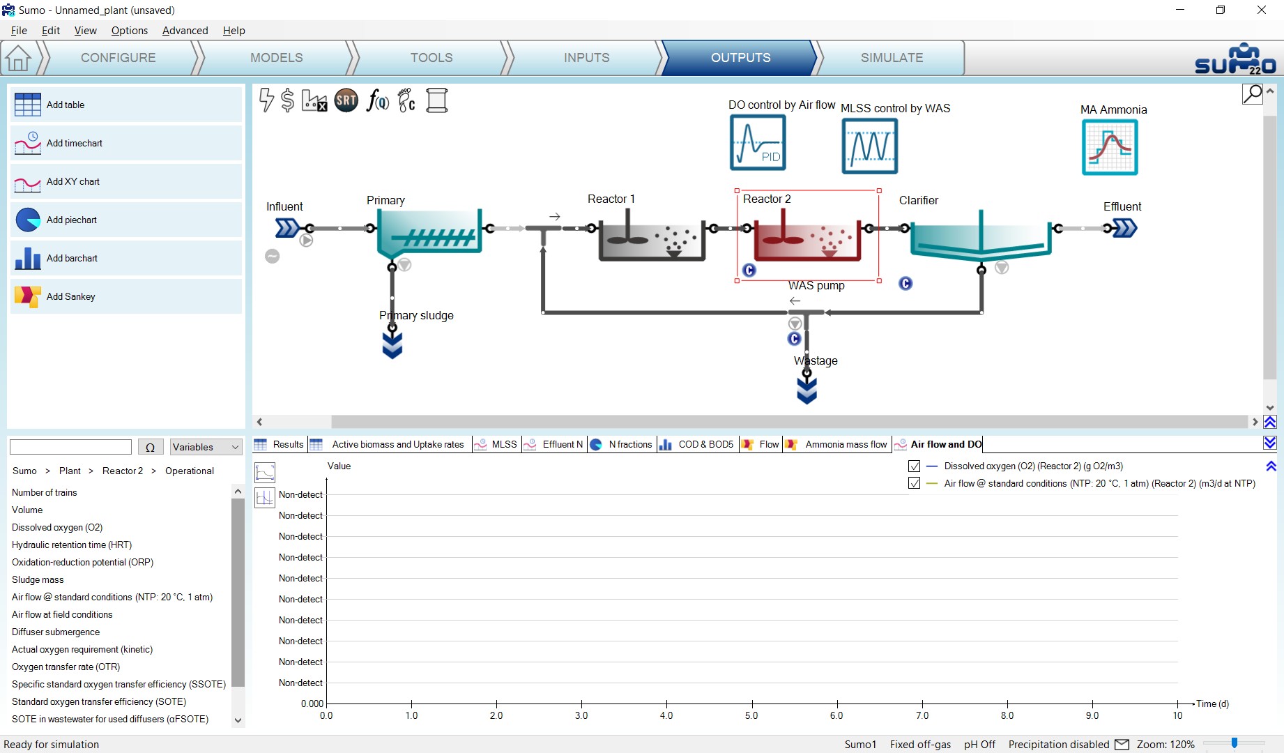
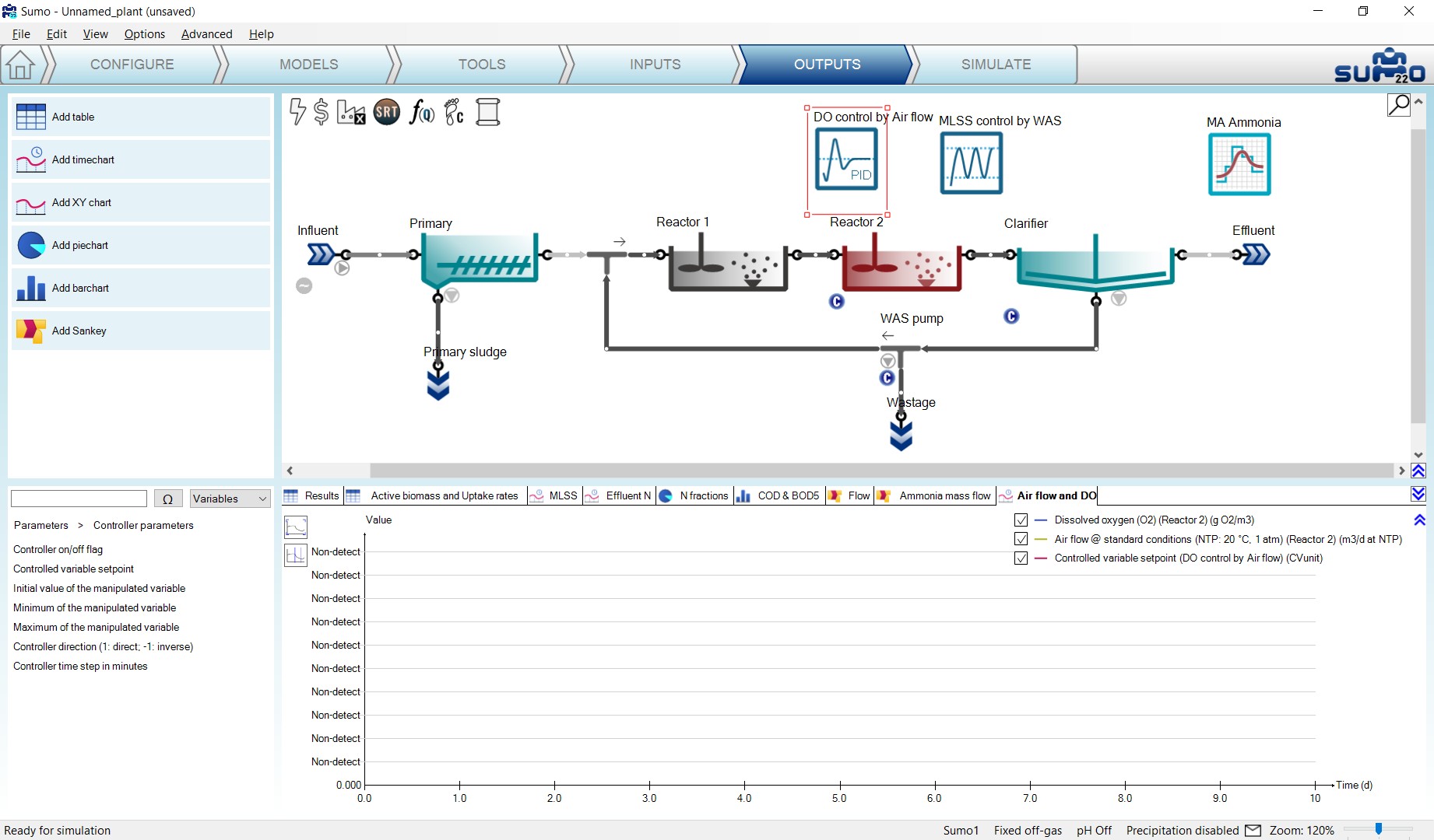
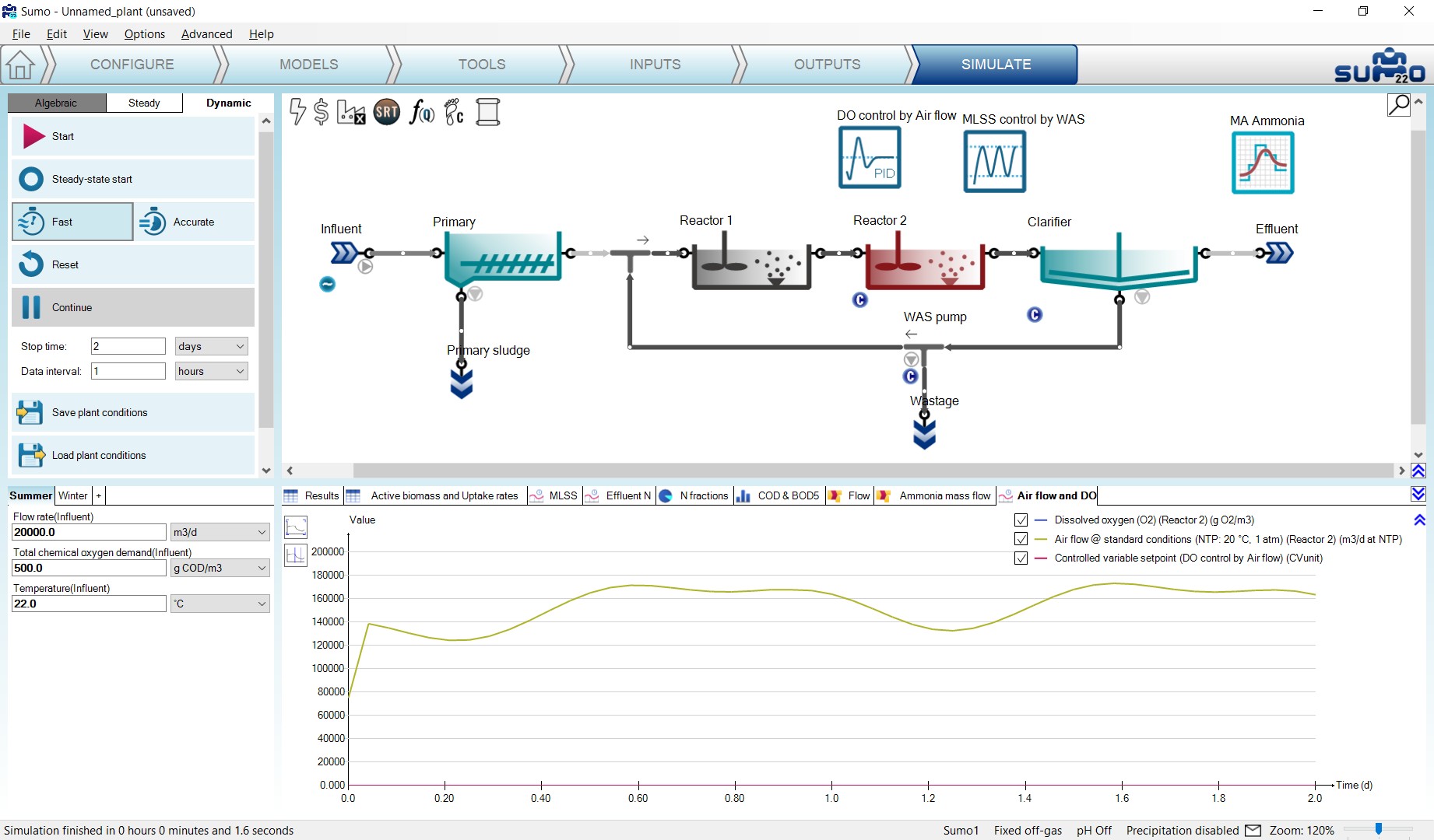
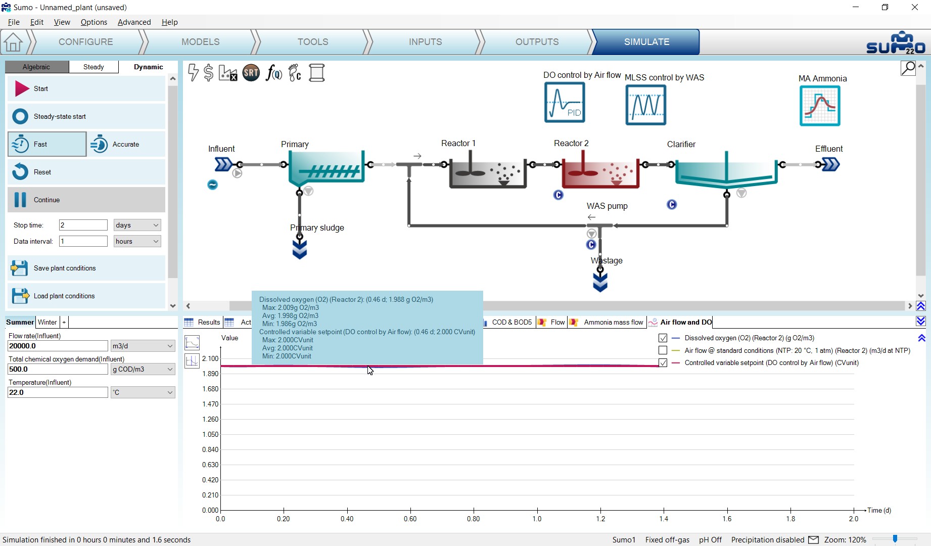
Switch on the diurnal flow dynamic input table for the influent on the Inputs/Dynamics tab, then go to the Simulate tab and set the stop time to 2 day, then run a dynamic simulation. During the calculation, you can follow the change of the air flow on the Air flow and DO timechart (Figure 4.13). Unchecking the Air flow item on the timechart, only the dissolved oxygen setpoint and the predicted DO will be shown (Figure 4.14). Using these gain settings, the controller can keep a strict fit to the setpoint without oscillation or overshoot (this can be verified by hovering the mouse on the graph and checking the values on the popup that appears on the timechart).
Note: It is good to keep in mind that this plant is subjected to dynamic influent load and a Deadband MLSS controller, thus the system never reaches steady state conditions.
¶ Ratio controller
The Ratio controller is using a ratio as multiplier for the manipulated variable, thus keeping the ratio of the manipulated and the control variable constant during the operation of the facility. To test this function, add a Carbon dosage unit (choose the mass flow based & methanol options) using a flow combiner before Reactor 1 of the example project, as shown by Figure 4.15 (renaming the new unit to “Methanol dosage”).
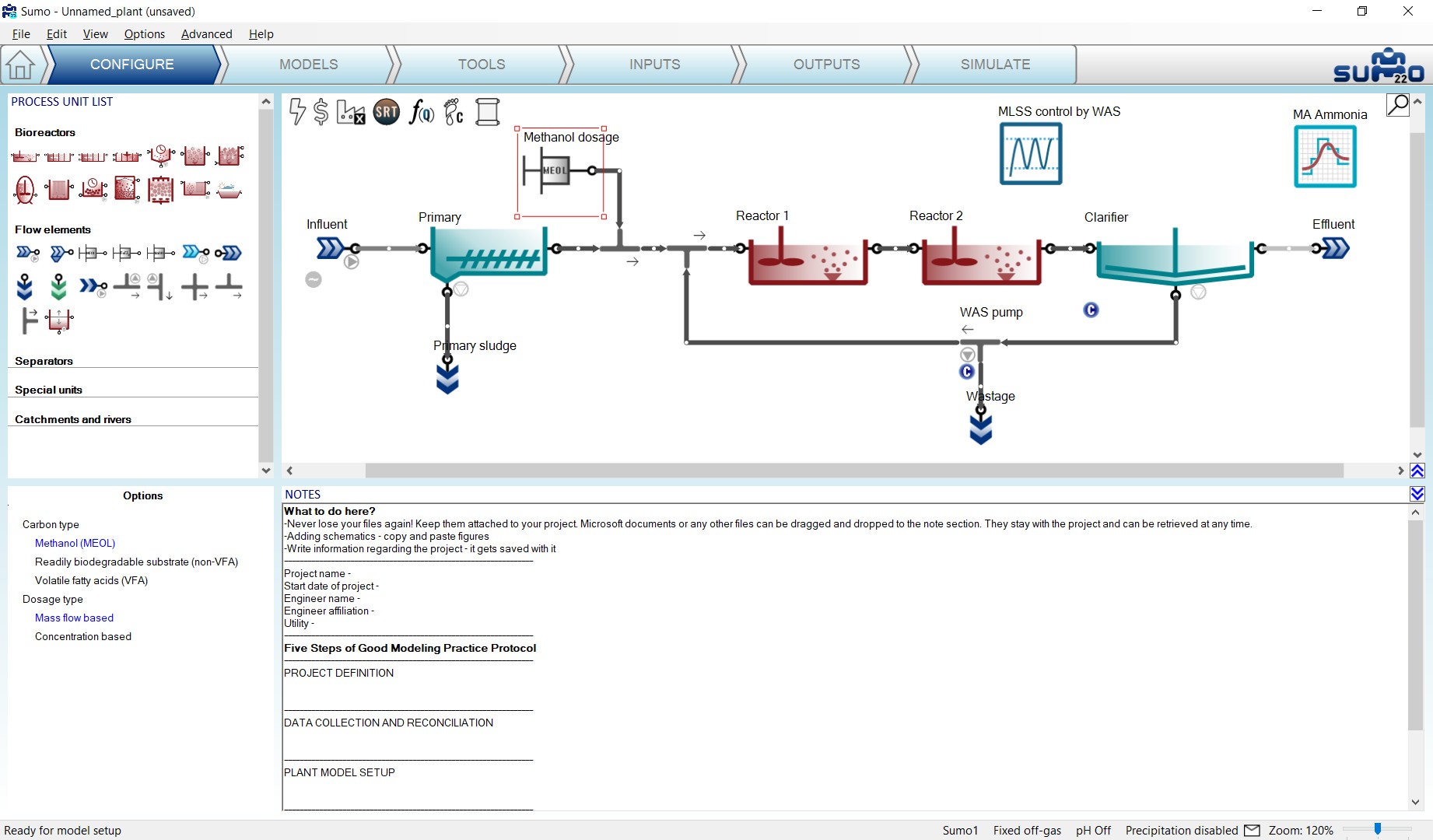
Now add the controller on the Tools tab as follows: first drag and drop the manipulated unit to the left side of the equation on the bottom right screen panel and the control unit to the right side of the of the equation. On the bottom left screen panel, you can now select the control variable and the manipulated variable of the selected units. In this example, we will manipulate the methanol dosage unit mass flow rate, depending on the ratio to the influent flow rate. Rename the controller (using F2 or right click) to “Methanol dosage control” (Figure 4.16).
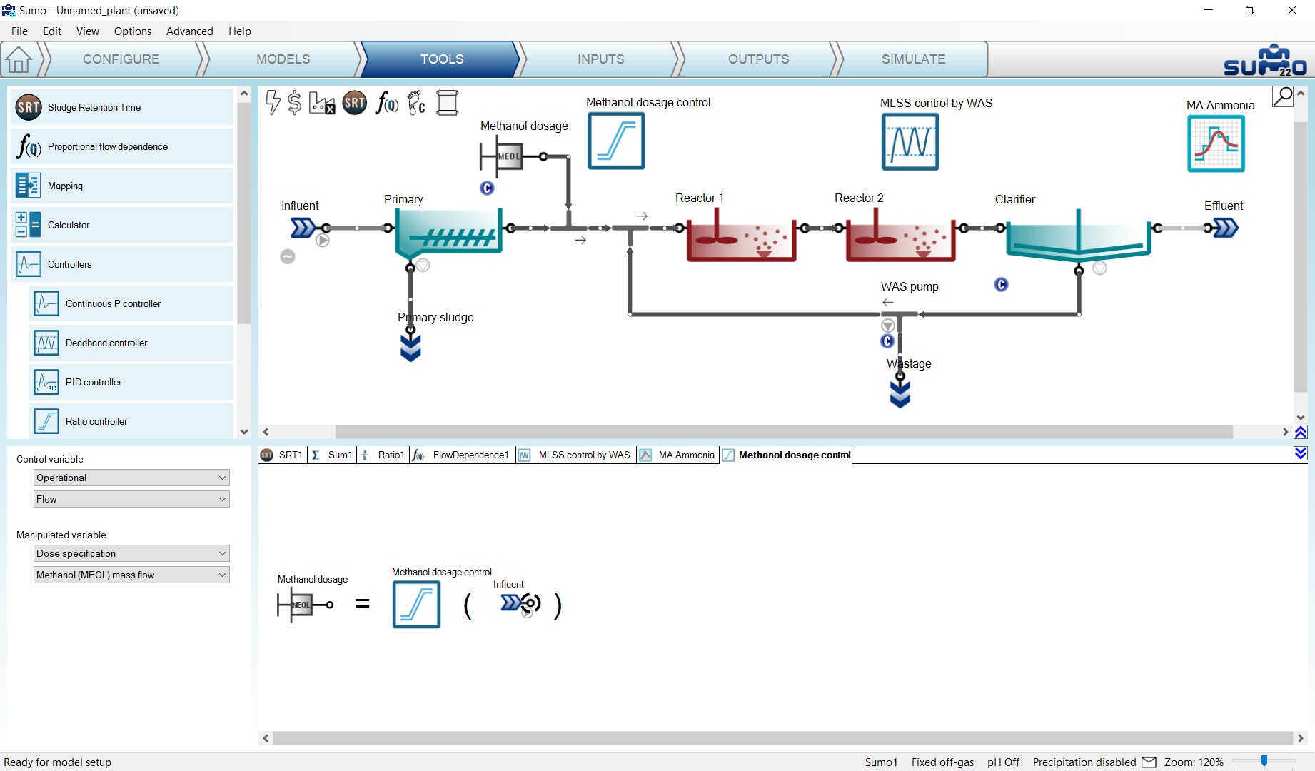
To properly set the controller parameters, the Unit system selection should be turned to “in code” in the Options menu > Unit systems. On the Inputs tab select the Methanol dosage and check the Unit of the mass flow – it is g COD/d (Figure 4.17). Select the new Methanol dosage controller. In the Ratio controller parameters table set the Ratio to 50, thus every influent m3 wastewater triggers 50 g of COD equivalent methanol dosage. Set the Minimum value of manipulated variable to 0, the Maximum value to 2.844E07 (equals the capacity of a dosage pump of 1 m3/h) and the Initial value to 1000000 (Figure 4.17). Turn on the dynamic input table for the Influent and leave other settings as they were set previously (Figure 4.17).

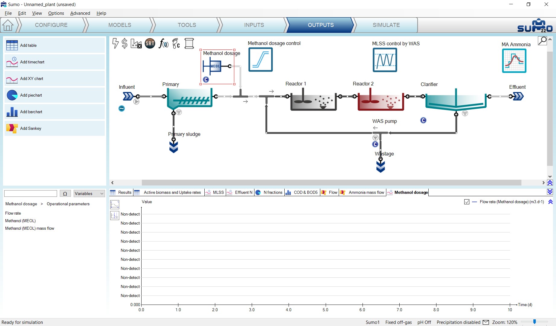
To follow the change of the Methanol dosage before Reactor 1, add a timechart on the Outputs tab and name it as “Methanol dosage”. Select the Methanol dosage process unit and drop Flow rate from the Operational parameters group (Figure 4.18).
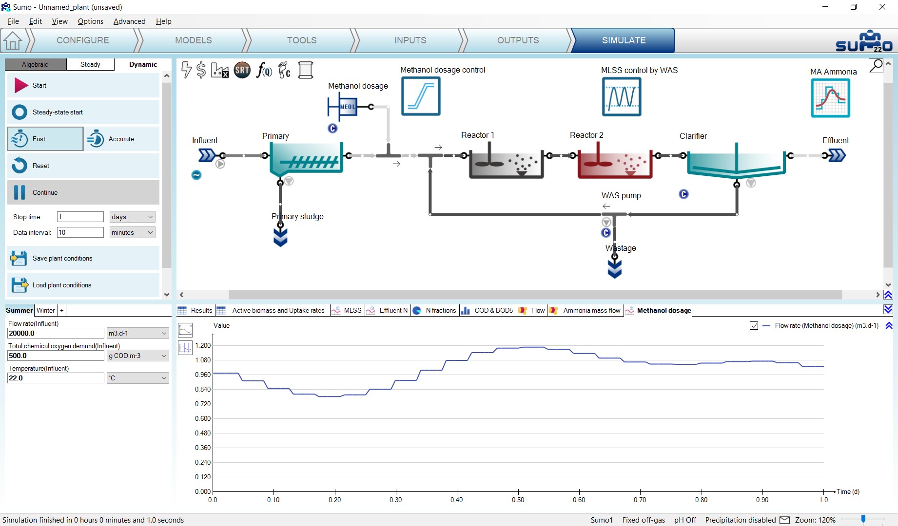
Go to the Simulate tab, set the stop time to 1 day with a data interval of 10 min and run a dynamic simulation. You can follow on the Methanol dosage timechart how the methanol dosage flow rate changes during the calculation, responding to the diurnal flow (Figure 4.19).
Now go to the Inputs and set the Controller on-off flag to 0 for the Methanol dosage control unit (Figure 4.20).

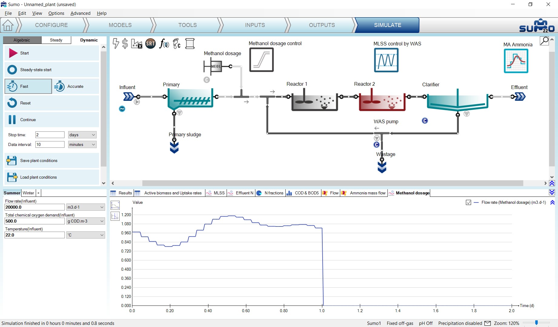
Go to the Simulate tab, set the stop time 2 days and hit Continue. The flow rate of the methanol dosage pump will drop to 0 m3/d (Figure 4.21), which corresponds to the value given at the Inputs/Constants tab as 0 g COD/d dosage rate. Note that the GUI turns the controller color to grey in order to inform the user that it is turned off.
¶ Time based on-off controller
The Time based on-off controller is a controller that sets the input parameter (manipulated variable) of the desired process unit based on a time step between a defined high and low value. This controller has no measured variable input (no control variable).
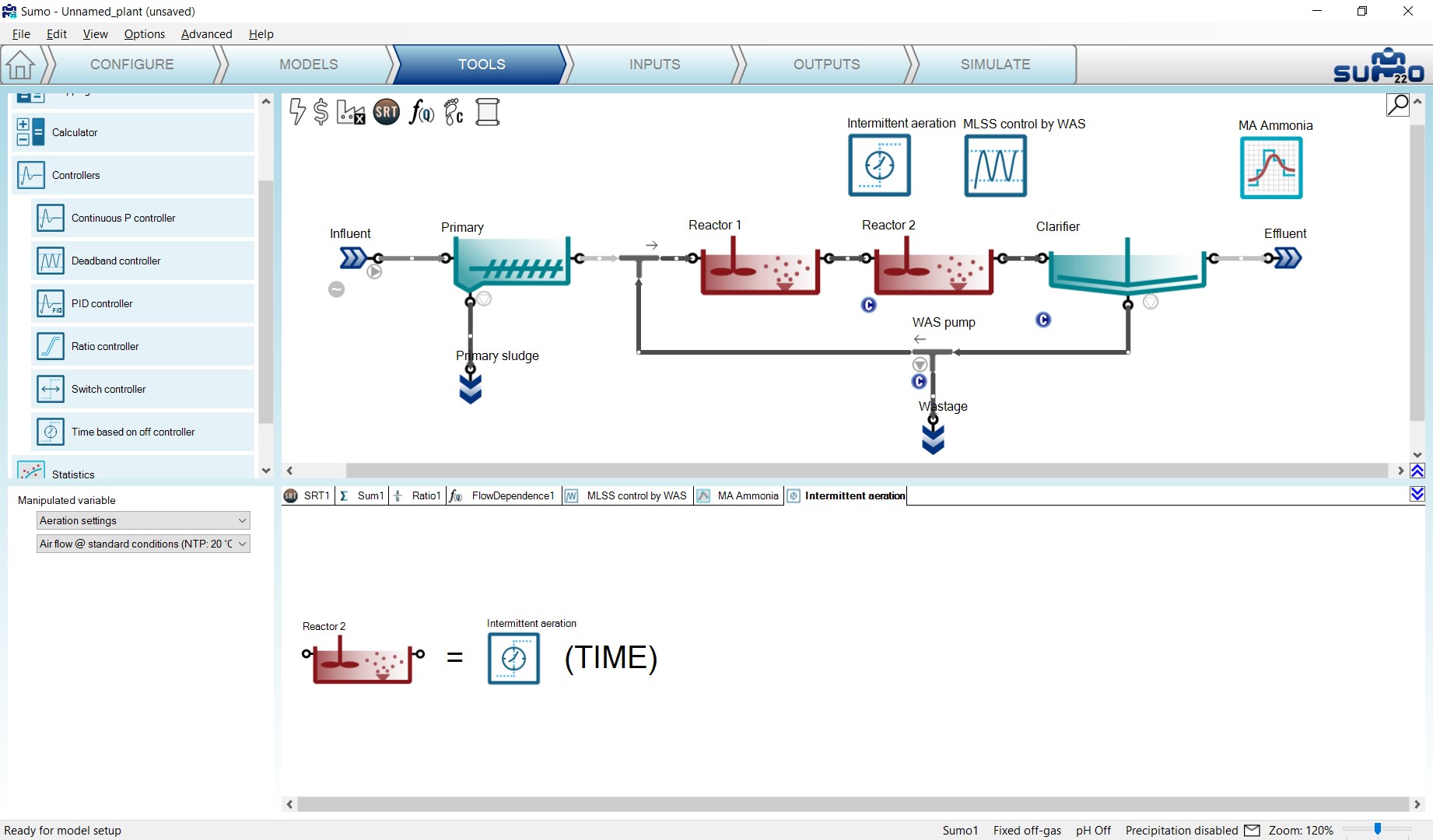
To demonstrate the capabilities of this controller, let us set Reactor 2 to use the Calculated option for Dissolved oxygen (Configure tab). Then add the controller and configure on the Tools tab as follows. First drag and drop the manipulated process unit (Reactor 2) to the left side of the equation in the bottom right screen panel. On the bottom left screen panel, you can now select the manipulated parameter of the selected unit. In this example, we will generate intermittent aeration in the chosen reactor by changing the air flow (located under Aeration settings). Rename the controller (using F2 or right click) to “Intermittent aeration” (Figure 4.22). This will rename the tab as well.
On the Inputs tab, select the new Intermittent aeration controller and review the Time based on-off controller parameters table. Set the Cycle length to 1 h, the Duration while the manipulated variable is set to high parameter to 0.5 h (aeration will be turned on for 30 min) and the High value of the manipulated variable parameter to 250000 m3/d, leaving the other parameters at default (Figure 4.23).

Before moving on, also make sure that the diurnal flow dynamic input table is turned on for the influent.
To follow the changes in the aeration of Reactor 2, add a timechart on the Outputs tab and rename it to “Air flow and DO”. Select Reactor 2 and drop Dissolved oxygen and Input air flow from Operational menu (same method as described in the PID controller chapter, see Figure 4.11).
Now go to the Simulate tab, set the stop time to 1 day with 1 minute data interval and run a dynamic simulation from steady state. During the calculation, you can follow the periodic changes in the air flow on the timechart (Figure 4.24).
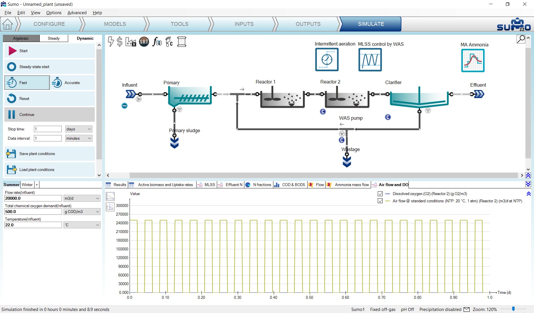
Unchecking the curve for the Air flow,in the legend, the resulting periodic changes in the dissolved oxygen can be seen in details. (Figure 4.25). The effect of the diurnal flow pattern can also be observed.
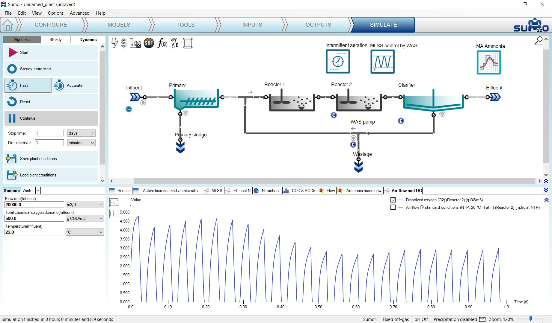
¶ Switch controller
The Switch controller is a controller that sets the input parameter (manipulated variable) of the desired process unit between two defined values (using an S-shaped function), depending on whether the control variable is above or below a defined threshold.
To demonstrate how this controller works, open the example project, add the controller and configure on the Tools tab according to the following. First drag and drop the manipulated process unit (Reactor 1) to the left side of the equation in the bottom right screen panel, then drag and drop the control unit (Effluent) to the right side of the equation. On the bottom left screen panel, select ammonia from the Frequently used variables as control variable and select air flow (located under Aeration settings) as the manipulated parameter. We will use this controller to apply intermittent aeration in the chosen reactor in order to meet the desired effluent ammonia concentration. Rename the controller (using F2 or right click) to “ABAC” (Figure 4.26). This will rename the tab as well.
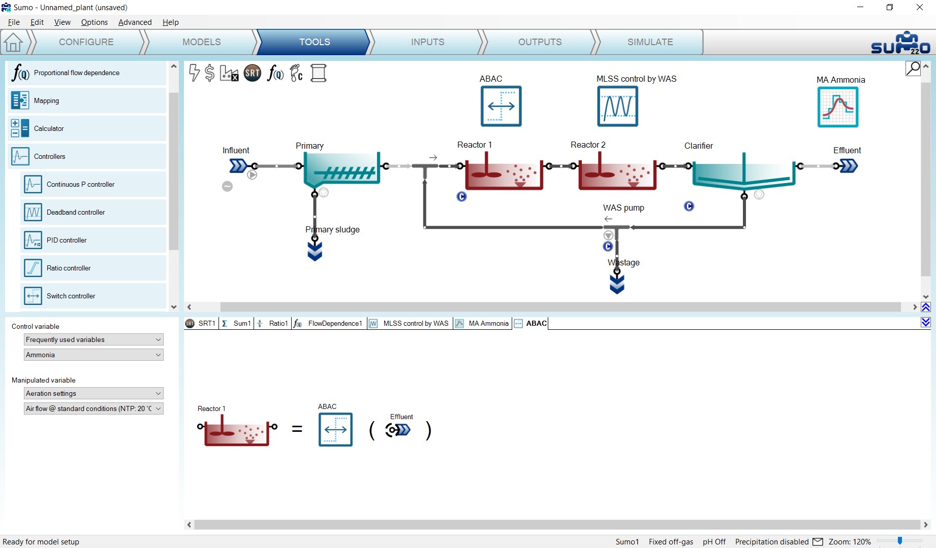
On the Inputs tab, select the new ABAC controller and review the controller parameters table. Set the Controlled variable threshold to 0.25 g N/m3 (this is a somewhat lower value than what the example layout could achieve for effluent ammonia), the Value of manipulated variable above threshold parameter to 35000 m3/d. By clicking on the Show all button in the bottom left panel, reveal Numerical parameters table and set the Slope of switch function to 0.0001 (this parameter sets the slope of the S-shaped function that is used by the controller). Leave all other parameters at default (Figure 4.27).

For this exercise, leave the diurnal flow dynamic input table for the influent turned off.
To follow the changes in the aeration of Reactor 1 and its effect on the effluent ammonia, add a timechart on the Outputs tab and rename it to “ABAC”. Select Reactor 1 and drop Dissolved oxygen and Air flow @ standard conditions from the Operational menu (same method as described in the PID controller chapter, see Figure 4.11). Then select the Effluent process unit and add Total ammonia from the Nitrogen components menu.
Now go to the Simulate tab, set the stop time to 1 day with 1 minute data interval and run a dynamic simulation. During the calculation, you can follow the periodic changes in the air flow on the timechart (Figure 4.28).
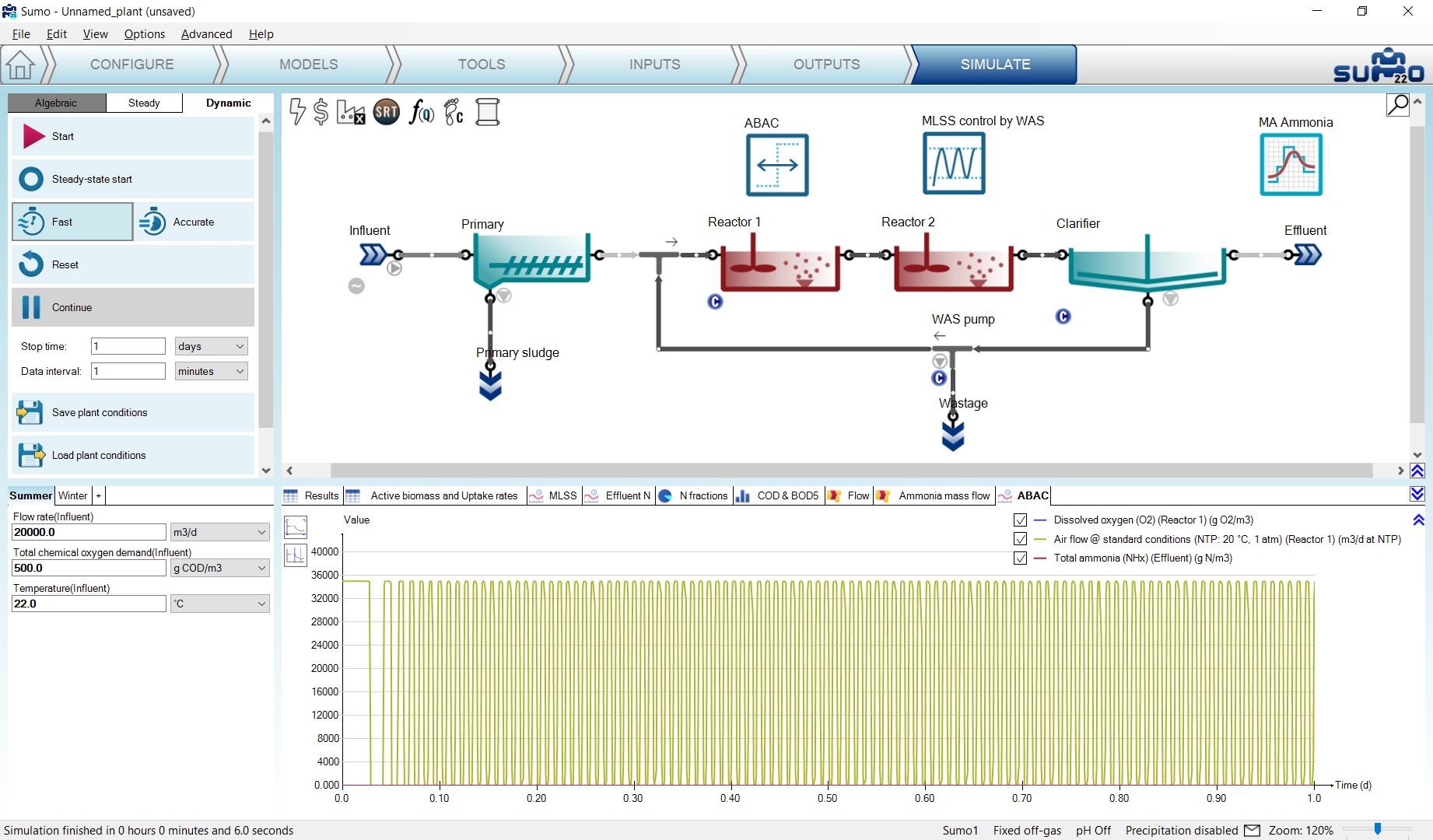
Unchecking the curve for the Air flow in the legend, the resulting periodic changes in the reactor dissolved oxygen and the effluent ammonia can be seen in details. (Figure 4.29).
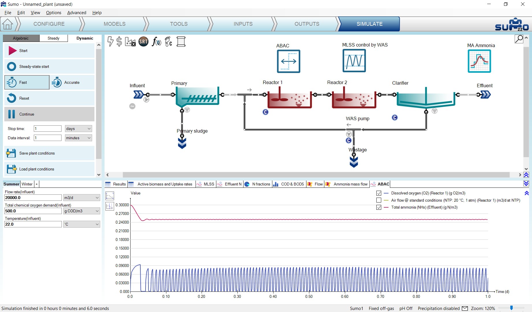
Now turn on the dynamic input table for the influent on the Inputs/Dynamics tab, increase the Value of manipulated variable above threshold of the ABAC controller to 70000 m3/d on the Inputs/Constants tab and run a new simulation from steady state. On the same timechart, you can follow how the controller adjusts the aeration in order to maintain the effluent ammonia concentration around the desired value despite of the diurnal flow pattern (Figure 4.30). As an exercise, you can investigate how the controller would work with the previous Value of manipulated variable above threshold setting and what effect would that have on the effluent ammonia.
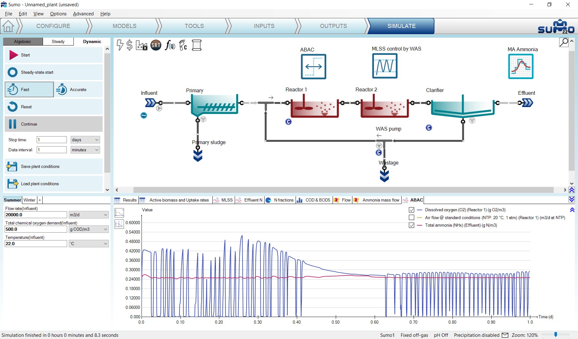
¶ Cascade controller
Cascade controllers can as well be set up in Sumo22, using the methods described above. To set up a cascade controller example, a PID and a Time-based on-off controller will be used in conjunction. Based on the time-based controller example it can be easily shown how the DO calculation effects the process in the reactors. To see the effect of calculated DO, the example prepared with the PID controller will be continued. In that example, the DO is calculated in Reactor 2 (Figure 4.31).
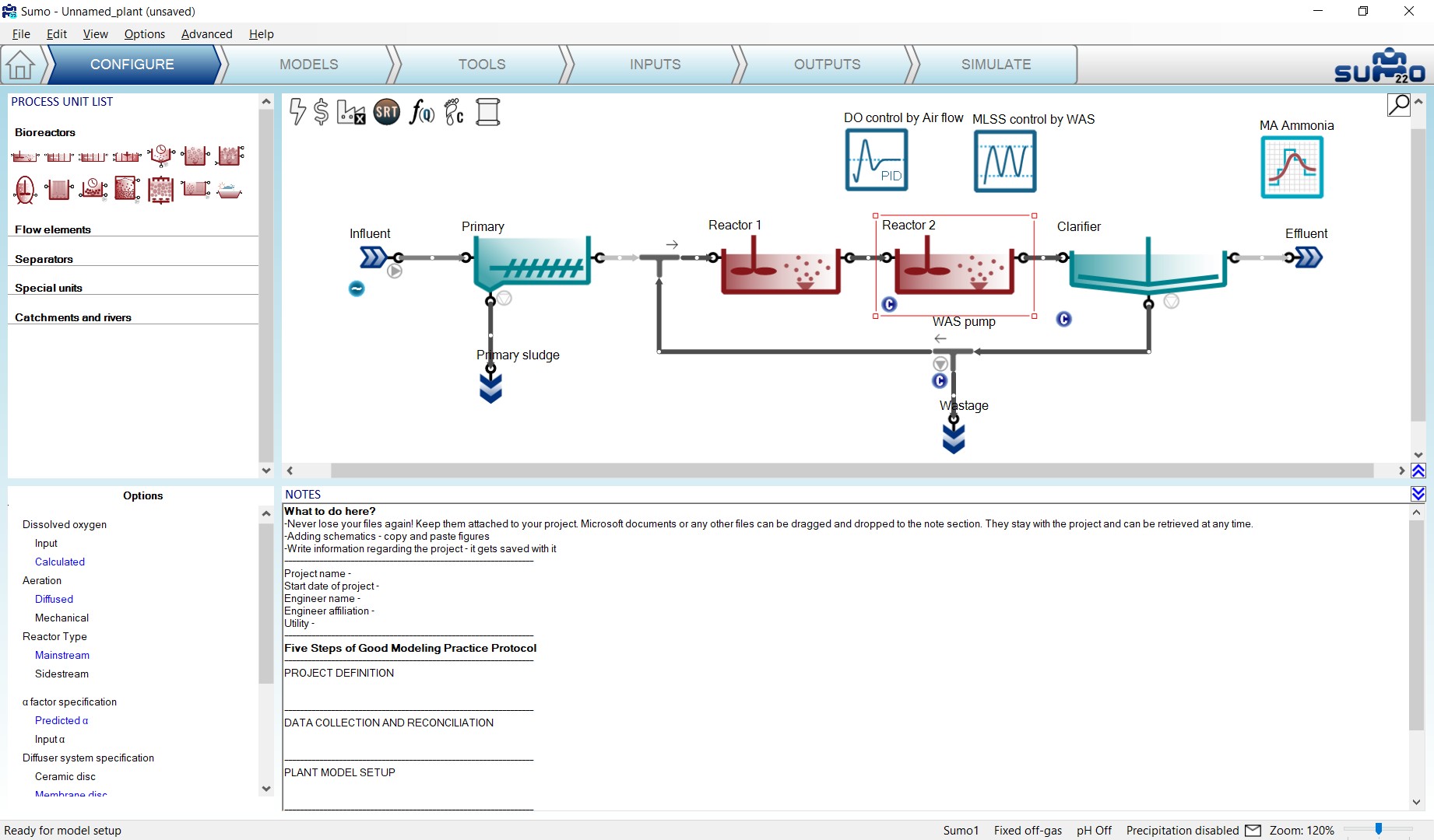
Go to the Tools tab and add a Time based on-off controller. In this example, we will generate a high-low setpoint, time-based aeration, by changing the DO setpoint, which is controller setpoint of the PID controller. To set up the Time based on-off controller, drag and drop the DO Control by Air flow controller icon from the drawing board to the left side of the equation in the bottom right panel and select Controlled variable setpoint from the Controller parameters menu in the bottom left panel. Rename the unit (using F2 or right click) – along with the tab – to “High-low setpoint aeration”. (Figure 4.32)
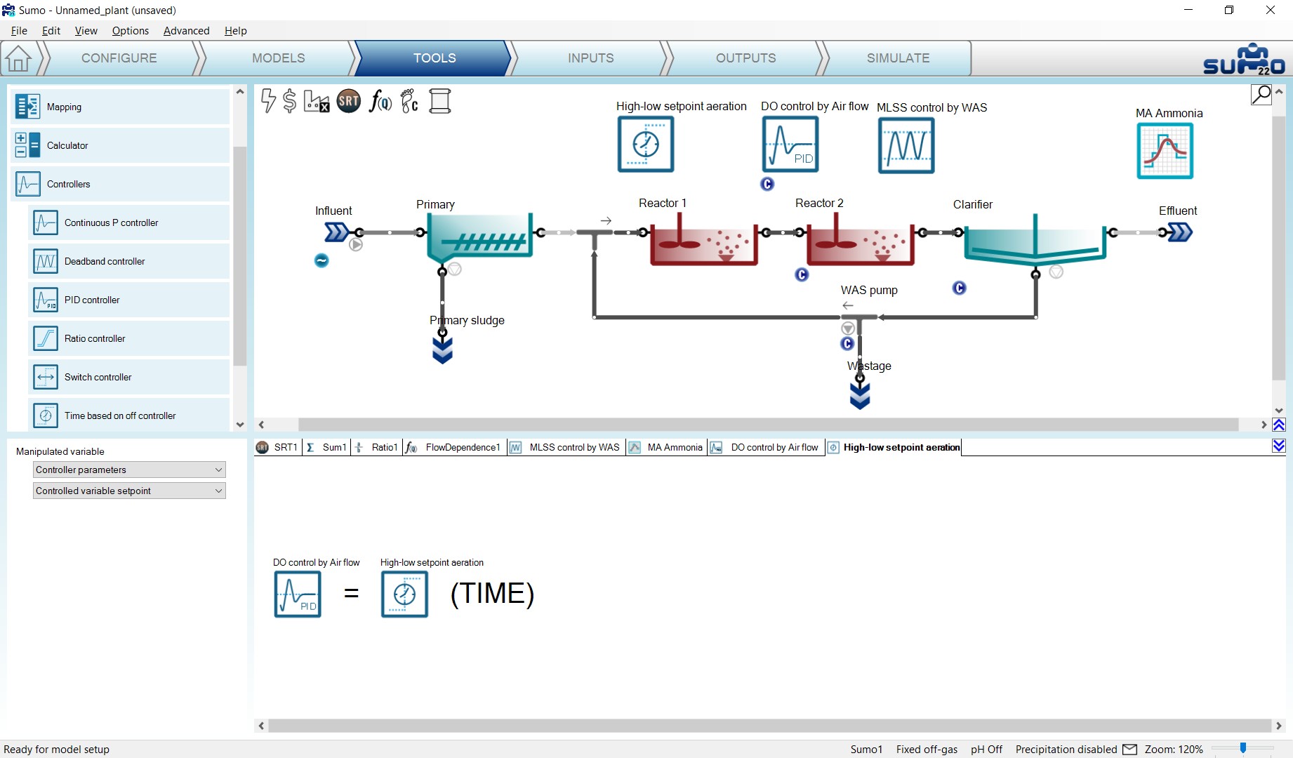
On the Inputs tab, select the new High-low setpoint aeration controller and in the Time based on-off controller parameters menu set the following (Figure 4.33):
- the Cycle length to 2 h (this is the default value),
- the Duration while the manipulated variable is set to high to 1 h (higher setpoint will be in effect for 1 h),
- Low value of the manipulated variable to 50% (or 0.5 without unit, depending on the Unit system settings), this equals 0.5 g O2/m3 as dissolved oxygen setpoint, and leave the other parameters as default.
Now select the DO control by Airflow controller and in the Controller parameters menu, set the Controller time step to 1 min (Figure 4.33).

Go to the Simulate tab, set the stop time to 1 d and the data interval to 1 minute and start simulation. Select the “Air flow and DO” timechart. The change of DO follows the aeration change controlled by the PID controller (Figure 4.34). Compare the new results with the results of the simple Time based on-off controller exercise on Figure 4.25.
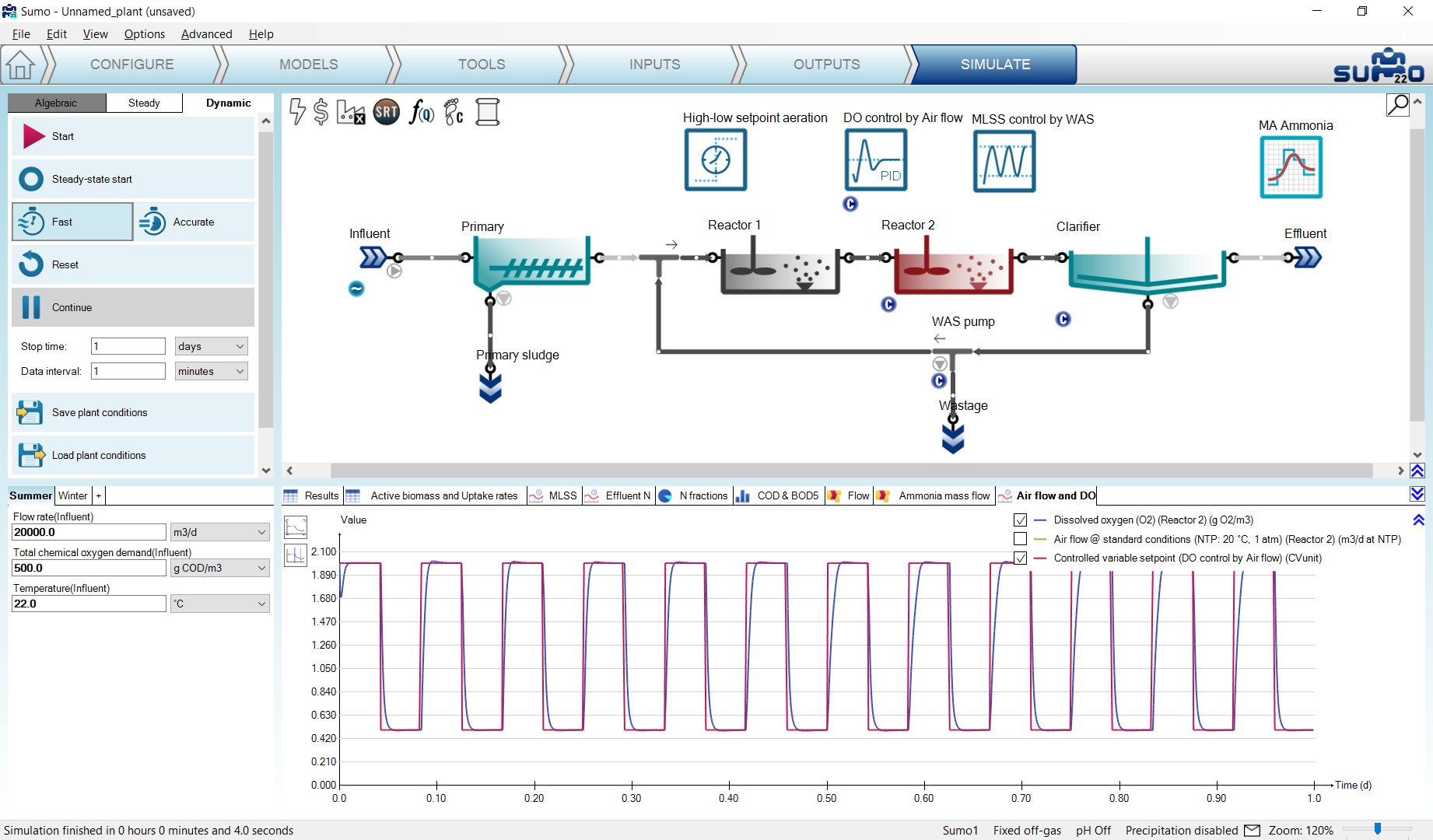
The change of Input air flow (Figure 4.35) shows a really different profile compared with the simple Time based on-off controller exercise (Figure 4.24).
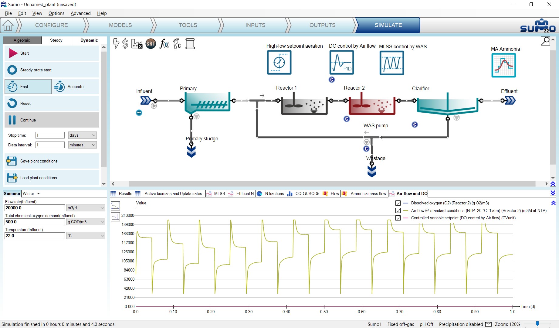
¶ Energy and cost calculations
Sumo features additional layers of energy and cost calculations, based on the process model. The energy mode can be used to assess the electricity demand of aeration, mixing, pumping and other equipment operation, as well as the available potential to produce electricity from biogas produced in digesters (enabling self-sufficiency assessment and scenario analysis for energy savings). The cost layer can be useful for evaluating and improving plant operation from an economic standpoint, by comparing the various cost items associated with the components of the energy balance and the usage of chemicals. In this chapter, an overview of the possibilities will be presented, based on the example project built in the How to use Sumo for simulations chapter.
The status of the energy and cost layers is indicated by the first two icons in the top left corner of the plant layout screen panel (Figure 5.1). By default, the energy mode is inactive and cost calculations are limited to basic inputs. While the energy mode is inactive, the cost center can be supplied with input data by selecting the $ icon in the Inputs tab. At this level, simple specific prices can be defined for electricity, water and polymer usage, as well as disposal fees and product sales (Figure 5.2).

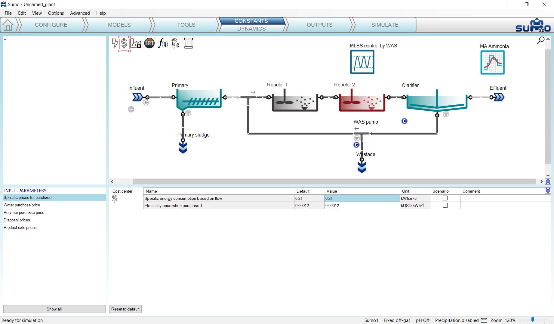
In order to fully exploit the capabilities of cost calculation, the energy mode shall be activated. This can be done by double-clicking on the Energy center icon (which will turn to yellow) or right-clicking and selecting “Turn Energy On”. Along with this, the Cost center icon will turn to black from hollow, and the specific price input options will also adapt to the energy mode (as well as the underlying cost calculations).
The Energy center plantwide input parameters are also available on the Inputs tab, by selecting the lightning bolt icon (Figure 5.3). Here you can specify general energy consumers that are grouped into periphery consumers (ventilation, water supply and miscellaneous), other variable and fixed consumers, as well as different on-site electricity producers and power storage options (depending on the settings of the Configure tab, see below).
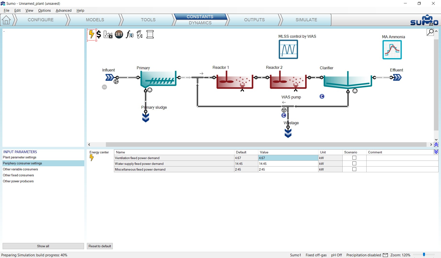
Apart from the plantwide inputs, the Energy center has a lot more to offer. Moving over to the Configure tab, you will see that the process unit library got extended with three new categories: Aeration units (blowers), Production units (biogas tank, CHP unit and flare) and Connectors (for gaseous phase flows – air and biogas). It is also on this page (in the bottom left screen panel), where you can specify whether the periphery power demands should be calculated based on PE (Population Equivalent) load, flow or entered directly in kW; as well as indicate whether the plant has PV units or batteries installed as on-site electricity production and storage options. (Figure 5.4).
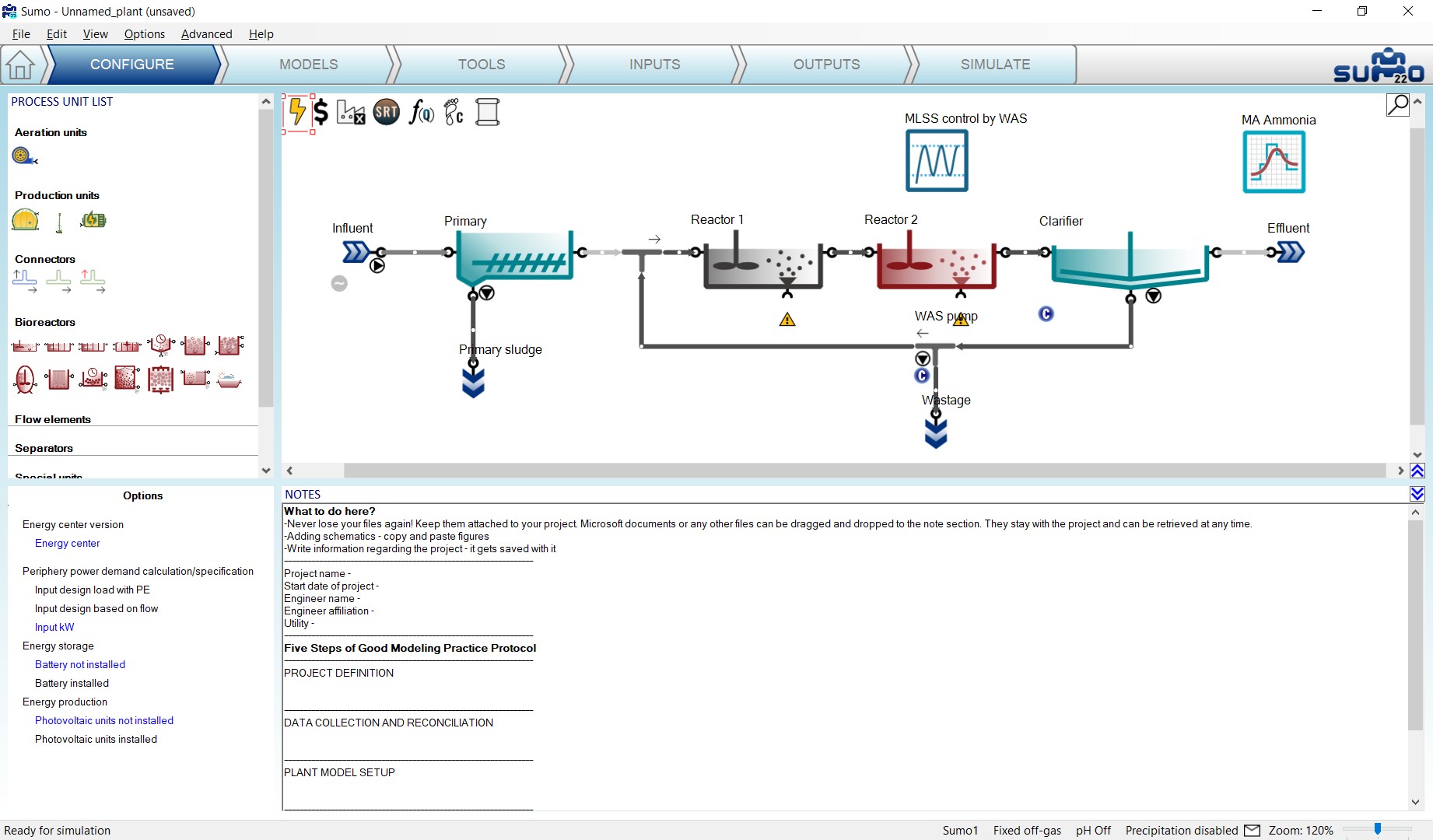
While on the Configure tab, let us extend the plant layout by adding a blower unit to the second reactor, connecting it to the air input port that appeared at the bottom of the reactor (Figure 5.5). Technically, we could attach another blower unit to the first reactor as well (or use an air connector unit to split the air flow from one blower to the two tanks), however, since it is not aerated, the air flow demand would be zero, thus there is no need for a blower there.
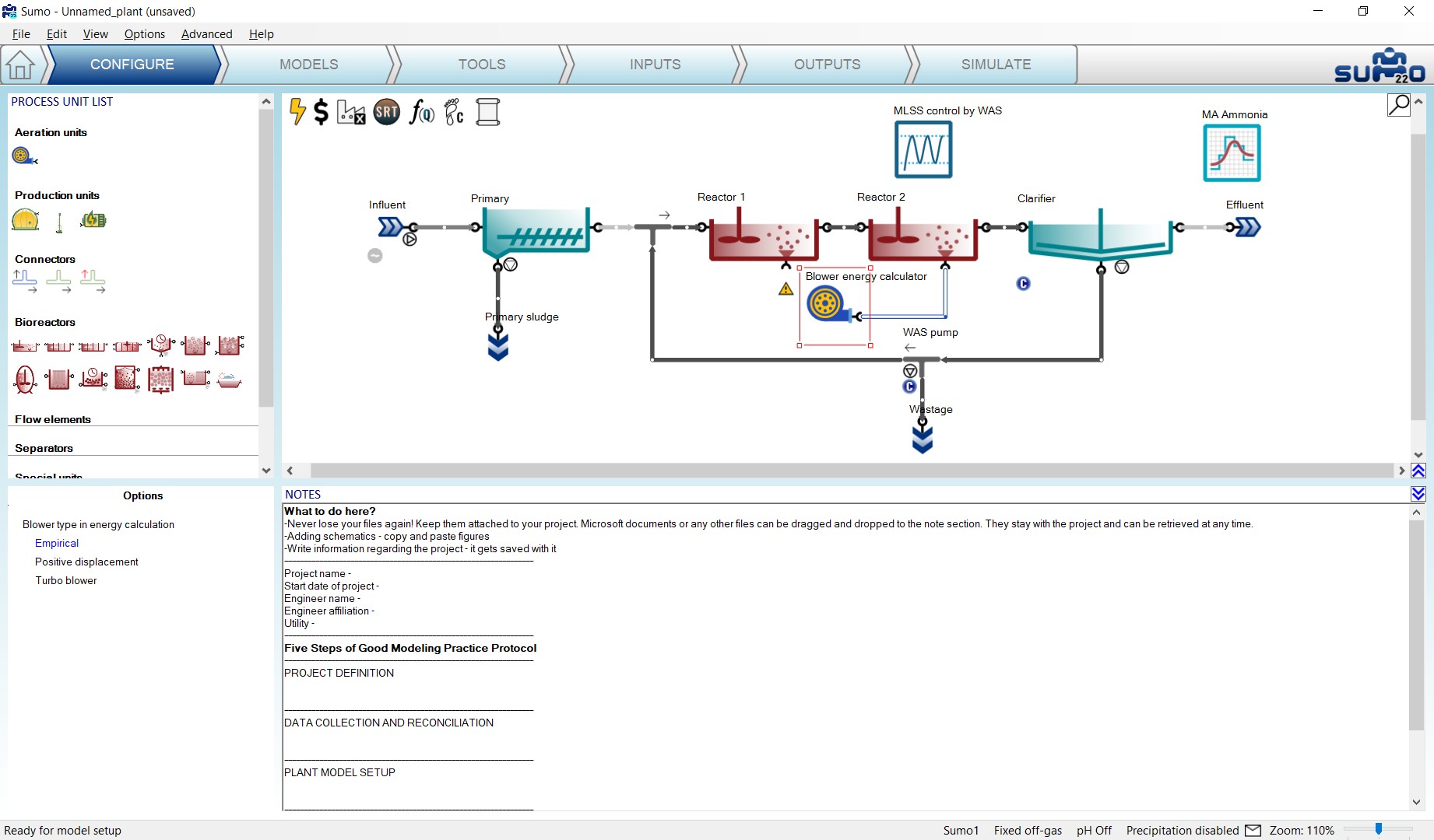
In the process unit options, you can specify between simple empirical (default), positive displacement and turbo blowers. The latter two come with delicate calibration tools that are available from the Inputs tab (just like the Influent tool), which offer full customization capabilities, based on blower manufacturer data. These tools are described in more detail in the Technical Reference. For our example, we will stick with the empirical blower.
You may also have noticed that the appearance of the pump icons by the influent, the clarifier and the flow splitter process units has slightly changed. When the energy mode is active, you can specify different pumping options for these process units in the bottom left screen panel; including gravitational flow (no pumping), empirical pump model (default), as well as more detailed centrifugal, displacement and screw pump models (Figure 5.6). The latter ones feature elaborate tools that are available from the Inputs tab, offering detailed pump customization based on manufacturer data. To learn more about these tools, the reader is referred to the Technical Reference. For this simple example, we will keep all pumps with the simple empirical model. It is also possible to assign pumps to the individual pipes by selecting them and specifying the pump type (there will be no visual notation of these pumps on the drawing board, but they will be included in the energy and cost calculations).
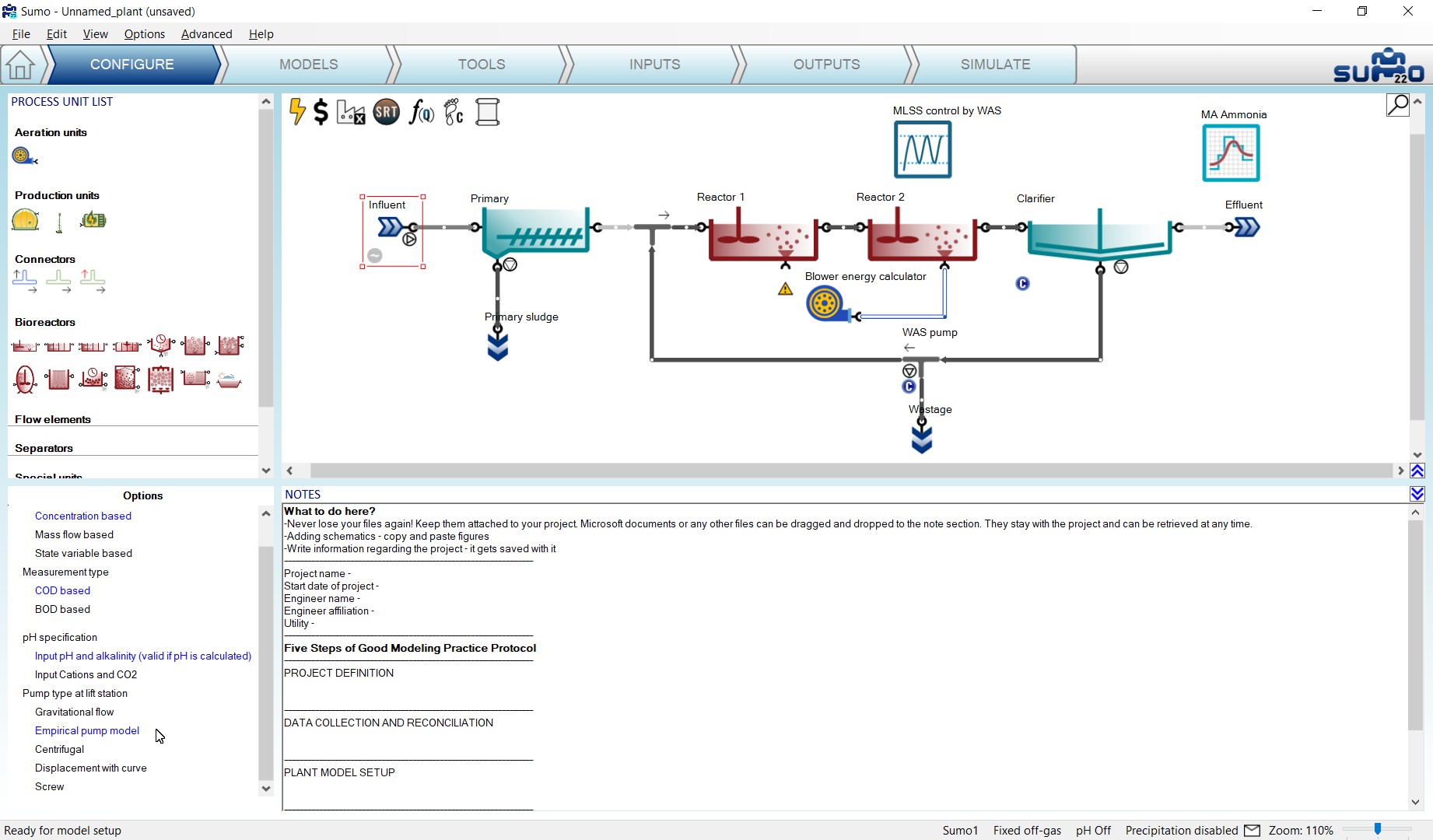
Moving over to the Inputs tab, the plant model will start to be recompiled (which is necessary for adding the extended features of the energy mode). The appearance of the pump icons will change from ‘not in operation’ to ‘in operation’ and the pump settings (in our example the efficiency) can be specified in the input parameters of the respective process units, one by one (as demonstrated for the influent on Figure 5.7). When using one of the detailed pump models, an extensive set of parameters will be available, to be used in conjunction of the respective pump tool.
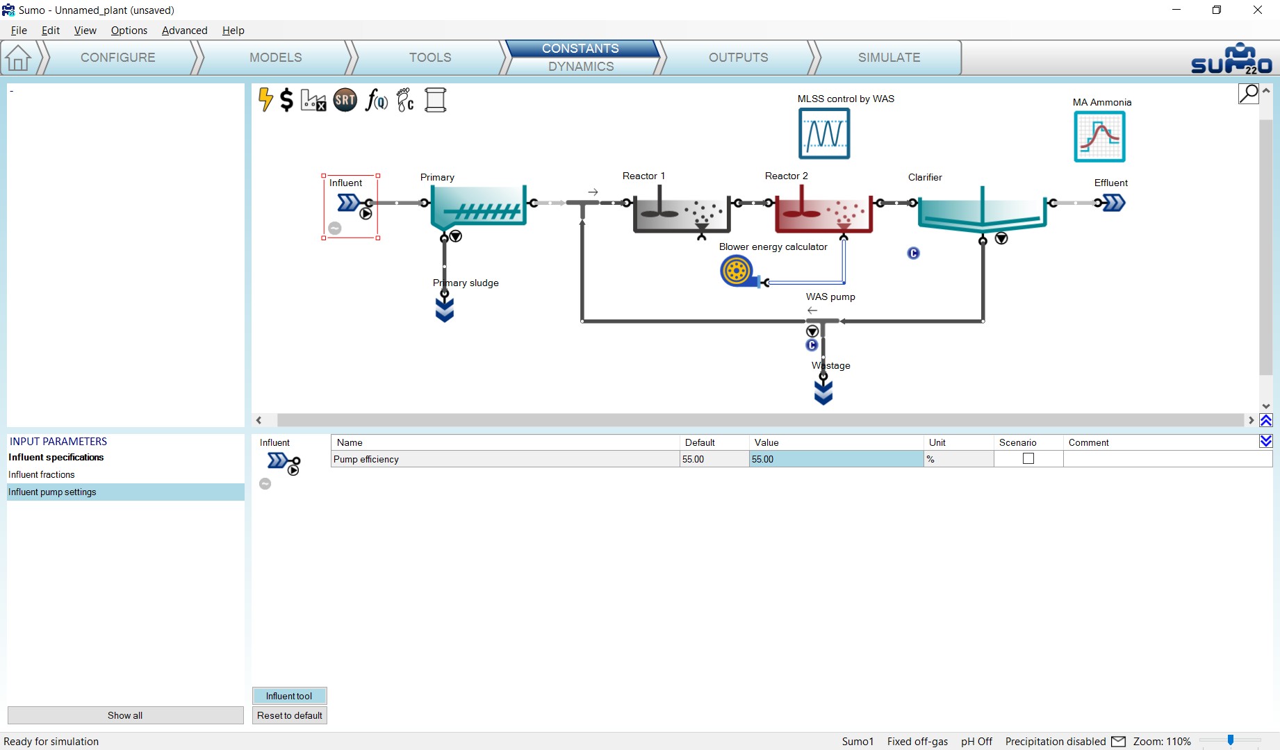
Similarly, the main input parameter for the blower in our example will be the efficiency, while selecting one of the more detailed blower models will require a range of additional parameters, whose proper calibration shall be performed using the respective blower tool.
Moving over to the Outputs tab, we can add various energy and cost related output information; such as a blower variables table by selecting the blower unit, adding a table and dragging over the variable group (Figure 5.8); an overview table of plant operation costs for the given simulation period by selecting the Cost center icon, adding a table and pulling the relevant variable group over on it (Figure 5.9); or piecharts showing the share of different energy consumer groups and categories in the plant by selecting the Energy center icon, adding piecharts and dragging over the respective variable groups to the charts.
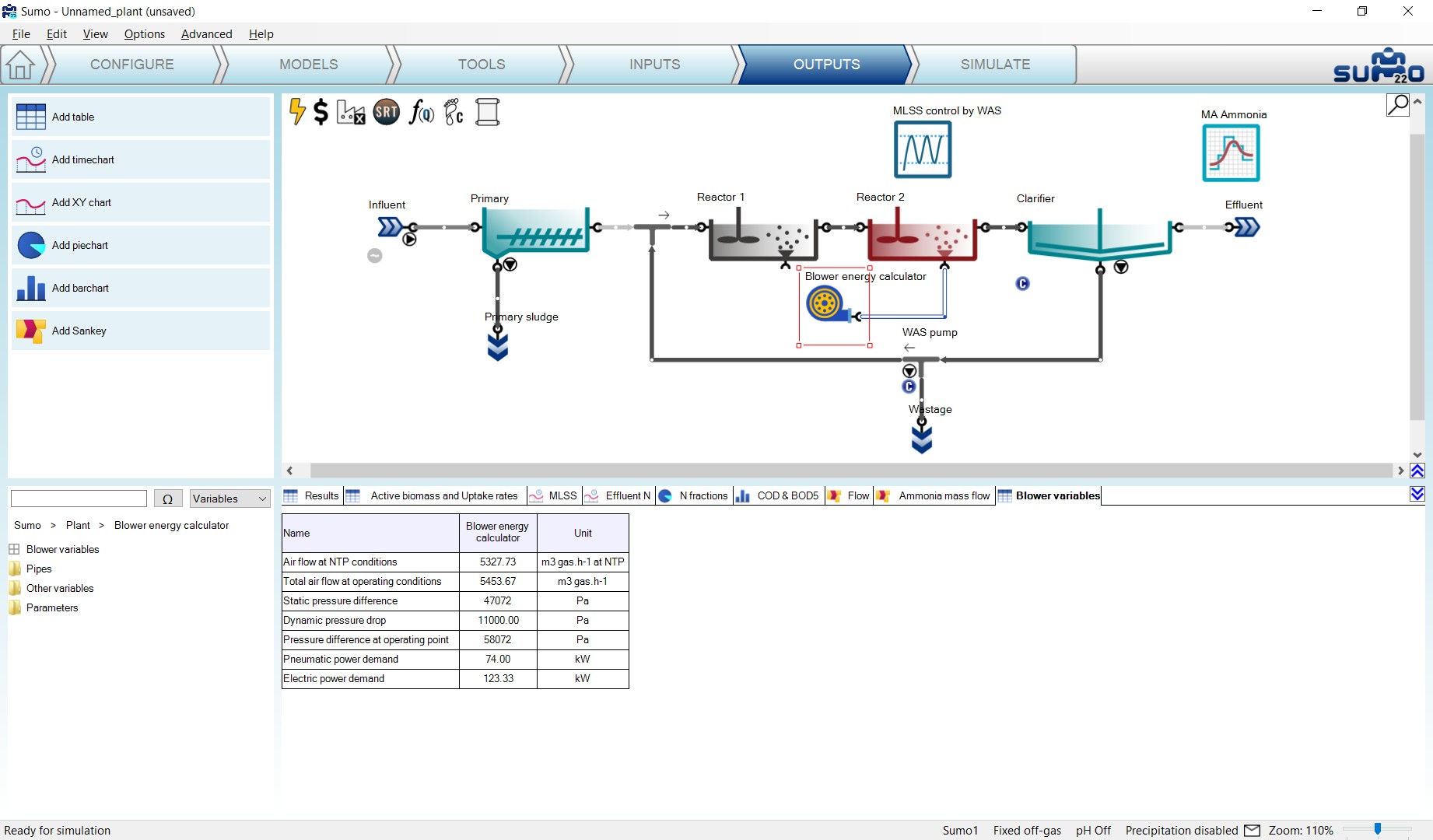
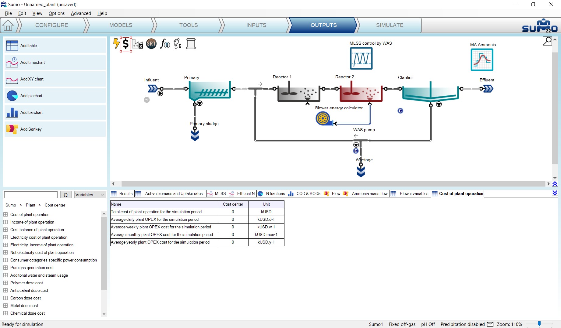
On the Simulate tab, after running a 30-day simulation from steady-state, you can review the energy and cost related information calculated by the model for this period. For example, it can be seen that most of the energy demand in this simple tutorial example comes from the electricity consumption of the biological treatment (Figure 5.10); basically aeration and mixing (Figure 5.11).
You can add various other energy and cost related outputs to analyze the performance of the plant in more detail, as well as extend the blower/pump models by specifying and calibrating the more detailed model options.
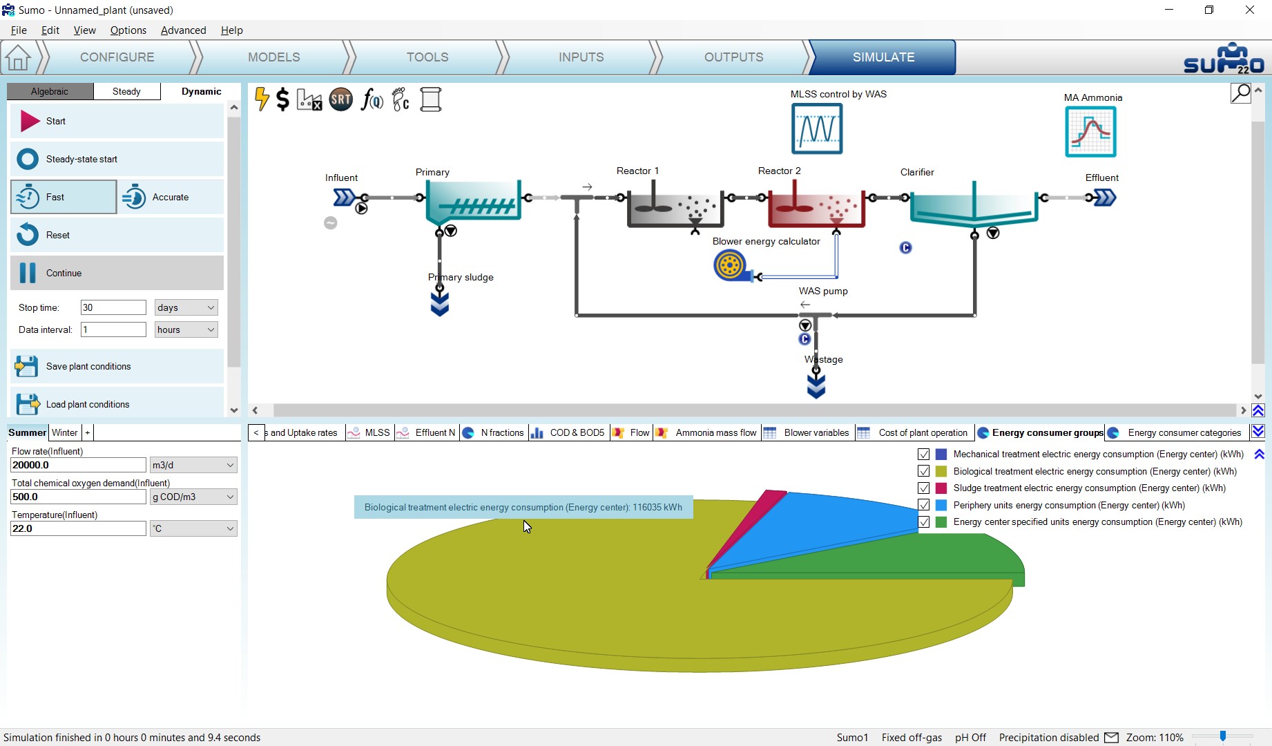
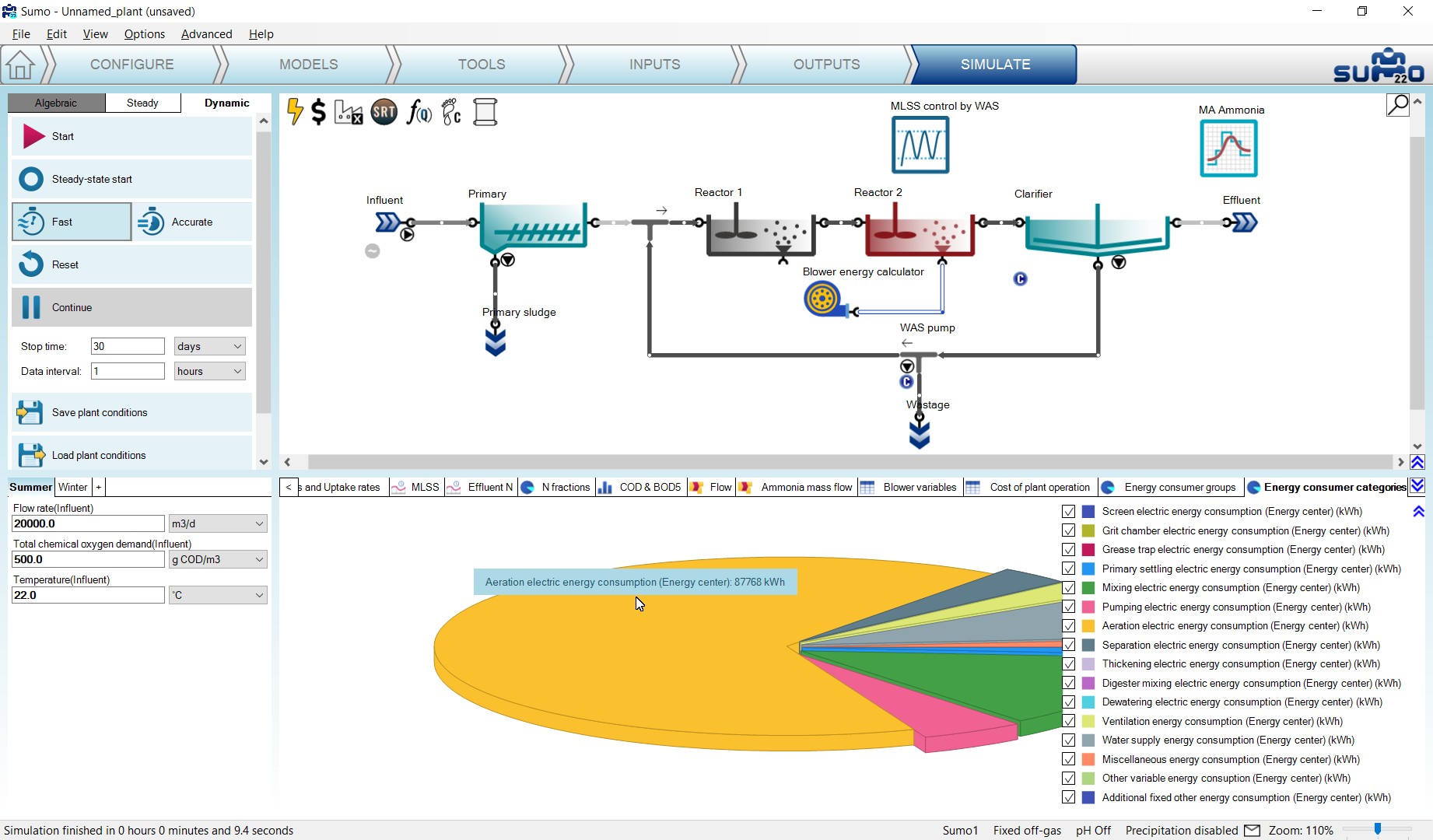
The usage of energy units associated with sidestream treatment (biogas tank, CHP unit, flare) is demonstrated by three of the factory examples: Tutorial Plant 2 with energy, AB plant with energy, UASB plant with energy.
¶ Carbon footprint calculations
This chapter will explain a new plantwide feature introduced in Sumo22. Using this feature enables the carbon footprint (CFP) assessment of plant operation for a given period, based on the process model and optionally, the energy calculations.
¶ Methodology
CFP assessment takes account of greenhouse gas (GHG) emissions related to the investigated activity. In the case of the wastewater industry the associated GHGs are CO2, CH4 and N2O (in general, there are number of other GHGs, however those are not characteristic of wastewater treatment processes). The assessment can address three levels, referred to as Scope 1, 2 and 3 (Table 6.1). Scope 1 covers direct GHG emissions originating from the processes, while Scope 2 and 3 deal with indirect emissions (the former is dedicated to GHG emissions pertaining to the supply of energy demands, the latter covers all other third-party GHG emissions, such as chemicals production, transportation of materials and personnel to and from the facility, etc.). By its nature, the choice of boundaries for Scope 3 can be very arbitrary, and often some crucial information elements needed for proper accounting are uncertain or biased. Thus, for comparative studies it is rather advisable to settle with Scope 1 and 2 carbon footprint assessment. The Sumo CFP tool provides these two levels.
Table 6.1 – Scopes of carbon footprint assessment.
| SCOPE 1 | Direct emissions from the investigated process |
|---|---|
| SCOPE 2 | Indirect emissions from energy consumption (imported power from external sources) |
| SCOPE 3 | Other indirect emissions associated with the process (external, third-party emissions) |
The status of the CFP calculation mode is indicated by the footprint icon in the top left corner of the plant layout screen panel (Figure 6.1). By default, CFP is disabled. To enable it, double-click on the CFP icon (whose image will change, depending on further conditions, see Table 6.2) or right-click and select “Turn carbon footprint calculations on”.

For carbon footprint assessment heavily relies on the proper estimation of off-gas mass flows, it is a requirement to have “Calculate gas phase concentrations” selected in the Gas phase category of Model options on the Models tab. As long as the “Input gas phase concentrations” option is selected, the CFP icon will be hollow red when turned on, indicating that an additional model option choice must be made before CFP calculations become active. With calculated off-gas, the icon will change from hollow to black fill and the letter ‘C’ on its right side will change to ‘S1’ (referring to Scope 1) or ‘S2’ (referring to Scope 2), depending on whether the Energy mode is switched off or on, respectively. Without energy calculations, the CFP calculations obviously lack the information needed for Scope 2 coverage, hence the two distinguished signals. Nevertheless, both levels of assessment will be valid for comparison with other assessments that were made on the same level.
Table 6.2 – CFP icon images shown under various conditions.
| CFP OFF | CFP ON | ||
| fixed off-gas | calculated off-gas | ||
| Energy OFF | Energy ON | ||
 |
 |
 |
 |
When enabled, CFP will automatically gather the following information from the various process units that are part of the plant layout:
- Stripping rates of GHGs from bioreactors and other process units with reactive volume
- Fugitive biogas mass flows from digesters and dewatering units
- Biosolids handling (assuming on-site incineration or transportation for off-site treatment)
- Incomplete biogas combustion (when the Energy mode is enabled)
- Energy consumption and production (when the Energy mode is enabled)
Regarding the process emissions, carbon dioxide and methane are always calculated based on the process model: stripped gas mass flows are fetched from liquid stream bioreactors, while fugitive gas mass flows are collected from solid stream bioreactors (digester, UASB) and dewatering units. In the case of nitrous oxide, the methodology depends on the process model used for the simulation. If the model includes N2O as a state variable (for an explanation of what is a state variable, please see the Technical Reference), then its emissions are calculated according to the process model, just like for the other two GHGs (Tier 1 method). Otherwise, N2O emissions will only be estimated based on the influent TKN via a plantwide emission factor (Tier 2 method), which, depending on the configuration, can be highly variable (0.01% - 1.8%, for details see Ahn et al, 2010). It is important to highlight that the choice between the two approaches is made automatically by Sumo, using a check in the actual process model. Therefore, it is generally advised to use a process model that has N2O as a state variable (e.g. Sumo4N, which can be found under Focus models on the Models tab) in order to avoid high uncertainty in estimating nitrous oxide emissions.
In the case of process-derived carbon dioxide, an important requirement is that a CFP assessment should only take into account the fraction of emissions that originates from the breakdown of materials containing fossil carbon (e.g. cleaning products, pharmaceuticals, and other petroleum-based products present in the wastewater). The CO2 produced by natural processes (originating from biogenic carbon) must be excluded. Therefore, estimating the share of fossil carbon is important in the various material streams of the plant. This can vary considerably, depending on the composition of the raw wastewater. Sumo considers default values for mainstream, side stream, biogas and biosolids based on literature. These can be adjusted/tuned by the user (e.g. for sensitivity analysis or for special applications).
In the final step of a CFP assessment, the emissions of GHGs are converted to CO2-equivalent units using a conversion factor called Global Warming Potential (GWP), which is provided by the periodically published official reports of the Intergovernmental Panel on Climate Change (IPCC). GWP values differ from one GHG to another (by definition, the GWP of CO2 is always 1, the values for all other gases are relative to this reference) and also vary depending on the reference time horizon chosen for benchmarking (100 years is the most often used period). GWP values based on the 100 and 20 years time horizons are presented by Table 6.3 to demonstrate the considerable differences between the three GHGs under investigation and also, to support the recommendation for using process model based N2O emission estimations (in a CFP assessment, 1 kg of N2O will be equivalent to about 265 kg of CO2 emitted).
Table 6.3 – GWP values (source: IPCC)
| GWP | Reference time horizon | |
|---|---|---|
| 20 years | 100 years | |
| CH4 | 84 | 28 |
| N2O | 264 | 265 |
Regarding the CFP of energy consumption, the assessment must consider the specific CFP of the utilized power generation approach (which is most often a mixture). Various technologies have quite different associated CFP per unit of power produced (see Table 6.4). Thus, the energy mix in general, and sometimes its temporal variation as well, is an important factor to take into account. Sumo offers a tool that serves as a database for properly setting up Scope 2 CFP calculations.
Table 6.4 – Typical specific CFP values for various power producing technologies
| Technology | Specific CFP [g CO2-eq/kWh] |
|---|---|
| Hydro | 24 |
| Solar | 45 |
| Natural gas | 490 |
| Wind | 11 |
| Nuclear | 12 |
| Coal | 820 |
¶ Usage
For the demonstration purpose we will use the “A2O with P recovery and energy plus CFP” example project, which is available on the welcome screen or from the Help menu.
After opening the example project, while on the Configure tab, select the Carbon footprint icon (located in the top left part of the layout panel) in order to look at the Process unit options. As CFP calculations are already turned on in this project, the process unit options are visible in the bottom left window panel. This is the place where the handling method of biosolids and the time horizon for GWP estimation base can be specified (Figure 6.2).
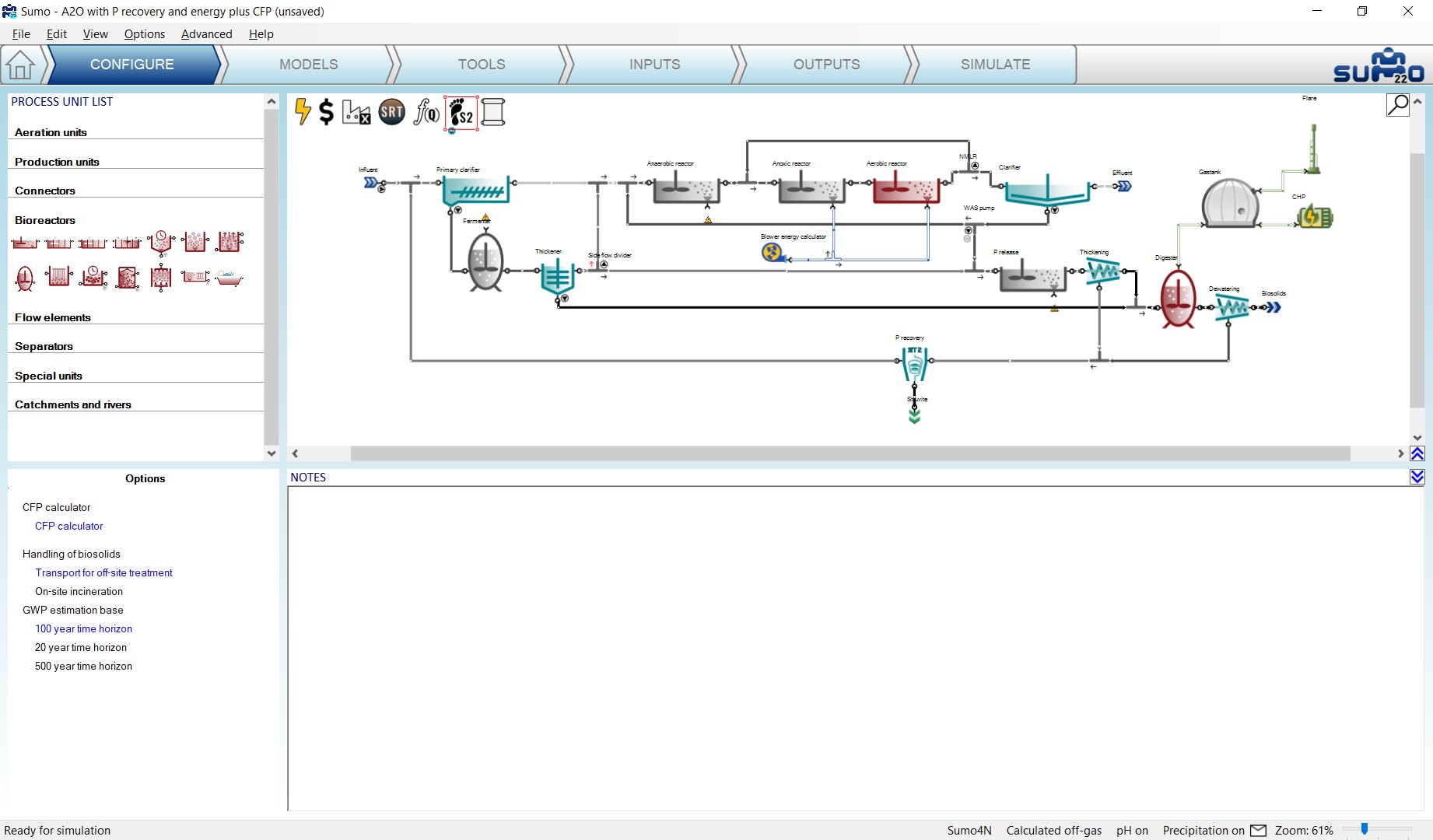
Moving over to the Inputs tab, the general input CFP parameters will appear. In the first table the Fossil carbon fractions can be specified (Figure 6.3). The second table contains the Sludge handling parameters (these depend on the previous choice of sludge handling method, see Figure 6.4). The third table contains the set of Electricity CFP parameters, which are used in conjunction with the Energy mode settings, enabling on-site and off-site power production methods (Figure 6.5). The latter table becomes active only when the Energy mode is turned on (enabling Scope 2 CFP calculations, like in this example project).
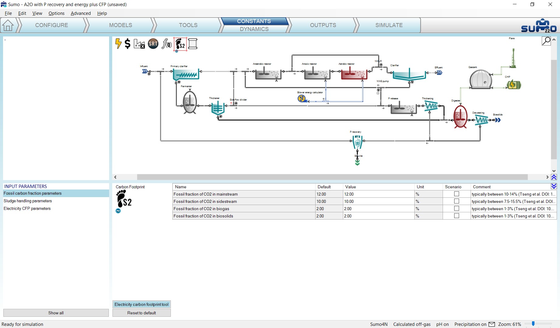
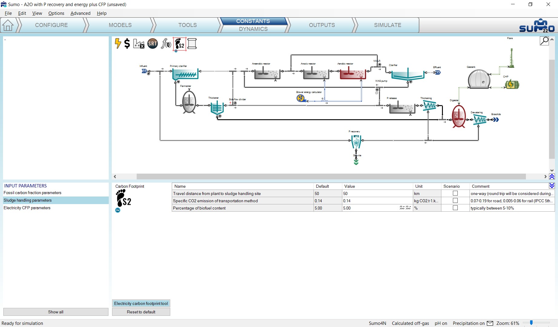
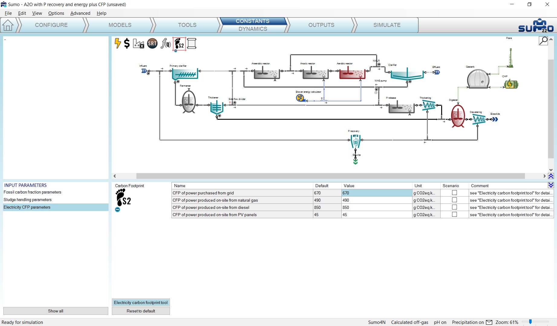
Below the parameter tables you can find a button for opening the ‘Electricity carbon footprint tool’, the database that is aimed to help determining correct grid and off-grid power CFP values, based on available regional and technology specific data. The example project uses one of the diurnal grid power CFP patterns from this tool (you can check it out by clicking on the Constants/Dynamics tab, see Figure 6.6).
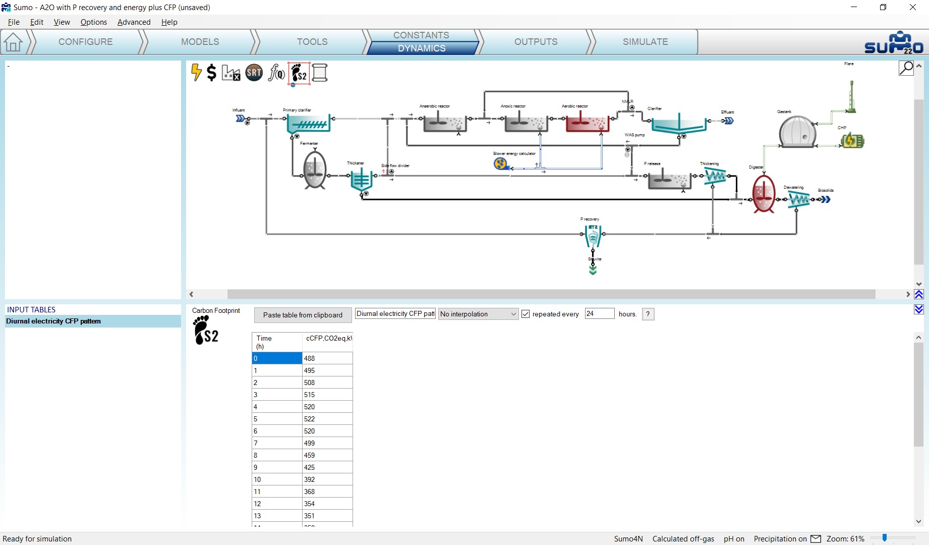
In order to assess all process-related CFP, new parameters have been added to the Digester and Dewatering process units. While on the Inputs/Constants tab, select the Digester on the drawing board and click the Show all button in the bottom left panel, then select the Gas phase settings table. You will find here the Fraction of fugitive biogas parameter, which has been modified in the example project from the default 0 to 1% (Figure 6.7). Similarly, when selecting the Dewatering unit, in the Settings table you will find parameters to adjust the fugitive mass flow fractions of methane and carbon dioxide (Figure 6.8).
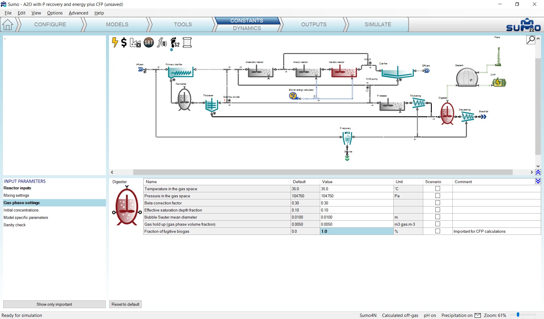
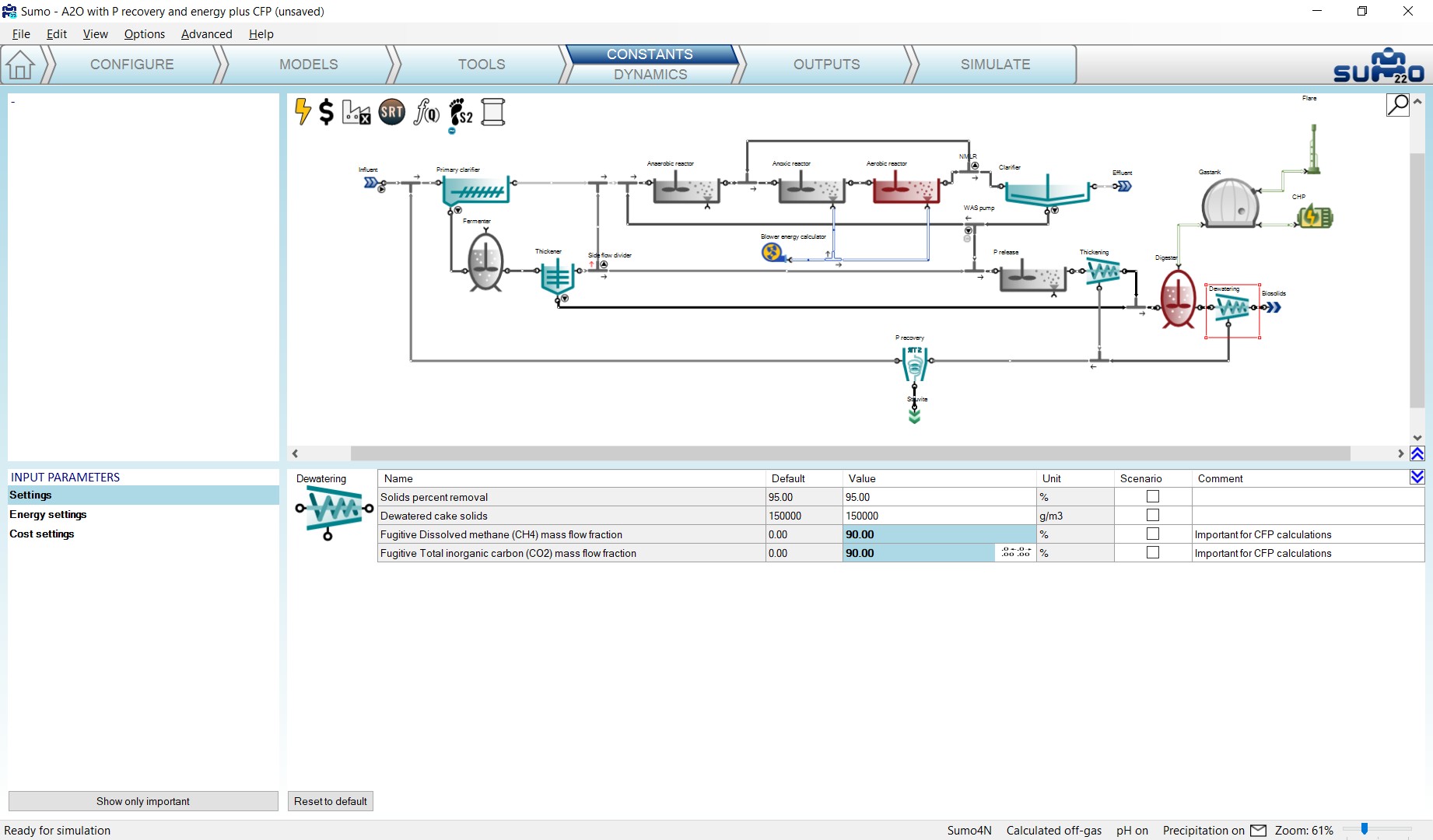
When Scope 2 CFP is enabled (Energy mode is active) and biogas processing is considered in the layout, it is also important to set the Combustion efficiency of methane parameter (available from the Combustion settings parameter table) in both the CHP and Flare process units (Figure 6.9). The value of this parameter is usually somewhere between 99% and 100%, which may seem indifferent, however, even such a little change in GHG emissions originating from incomplete combustion can make up a visible portion of the overall CFP.
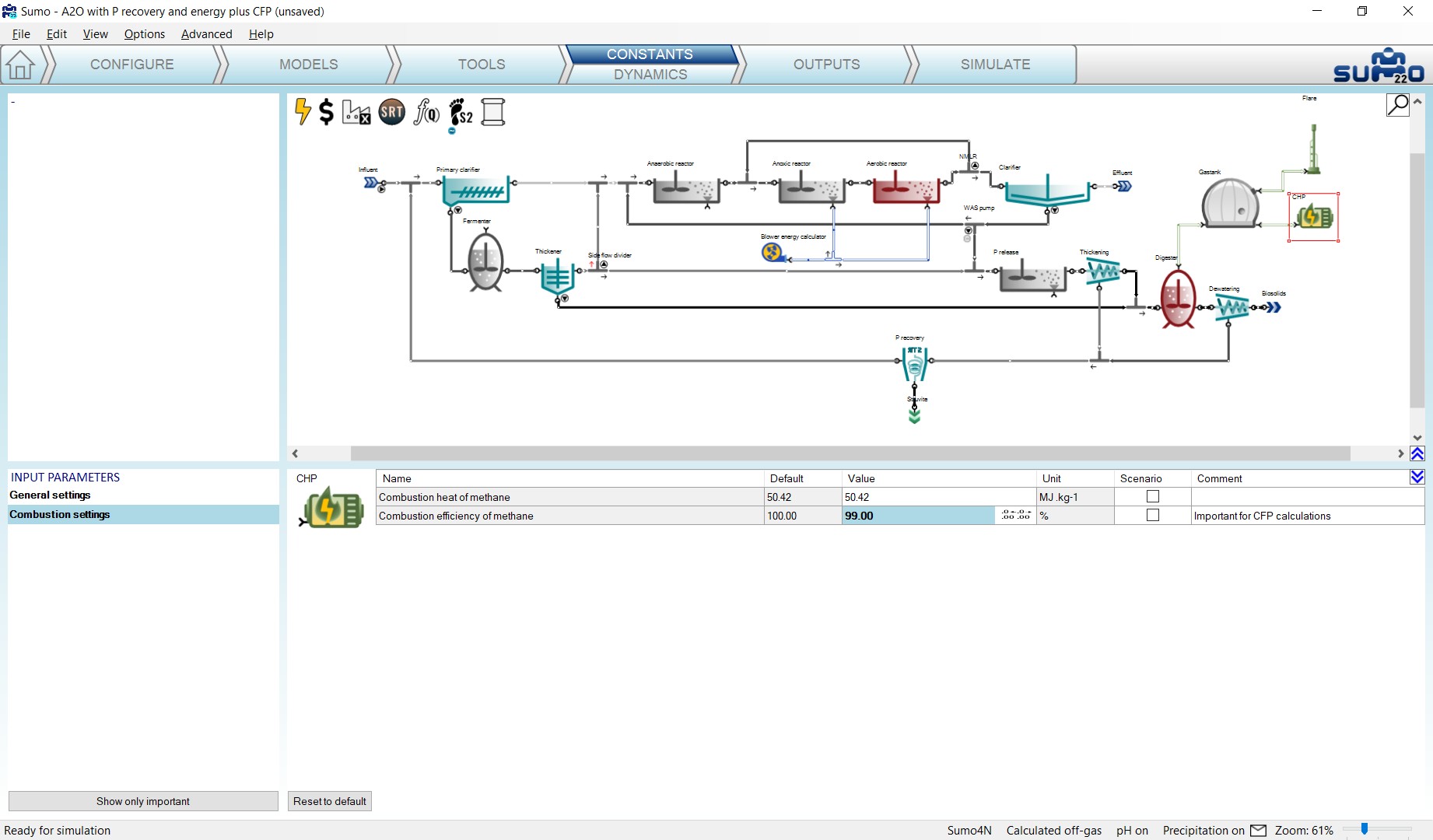
Results of the CFP assessment can be visualized by selecting the Carbon footprint icon on the Outputs tab and choosing from the prepared variable groups, such as ‘CFP summary’ or more detailed splits of direct and indirect CFP components, as well as CFP component splits focusing on the individual GHGs. Direct and indirect emission rates of GHGs are also available. To get some inspiration on how to use these data, proceed to the Simulate tab and launch a 1-day dynamic run from steady state, then review the outputs from the ‘CFP summary’ piechart to the ‘Electricity CFP’ timechart. From the ‘CFP summary’ (Figure 6.10) one can see that about two-thirds of the plant operation CFP for the simulated period comes from power usage, while the rest is about equally distributed between various process-related emissions of the three GHGs. Looking deeper, it turns out that about half of the overall plant operation CFP originates from the activated sludge process, while fugitive losses and incomplete biogas combustion, along with sludge handling (transportation to external handling site in this case) are smaller, yet visible fractions (Figure 6.11). The diurnal variability of electricity CFP is also visible but not outstanding (Figure 6.12).
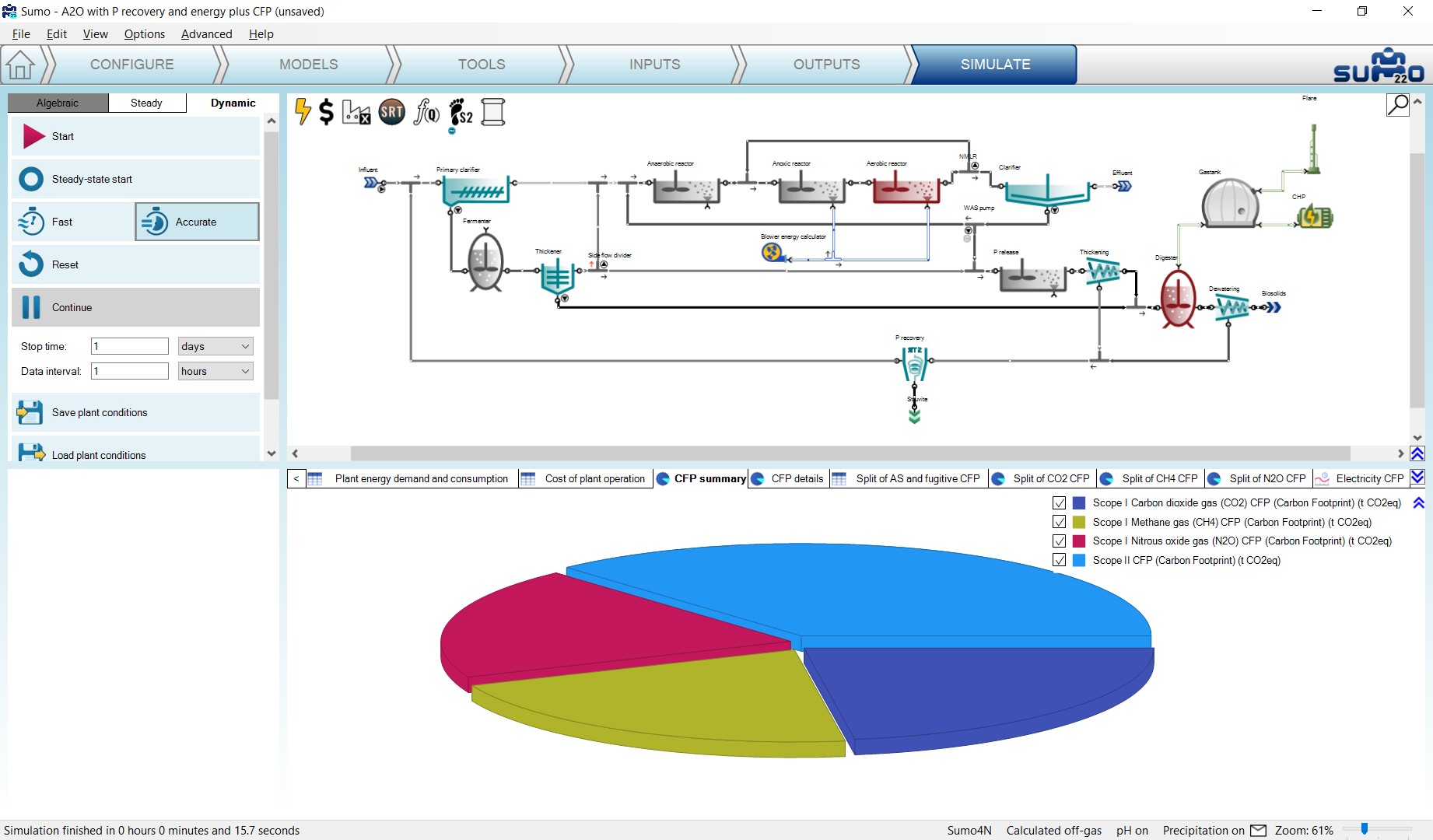
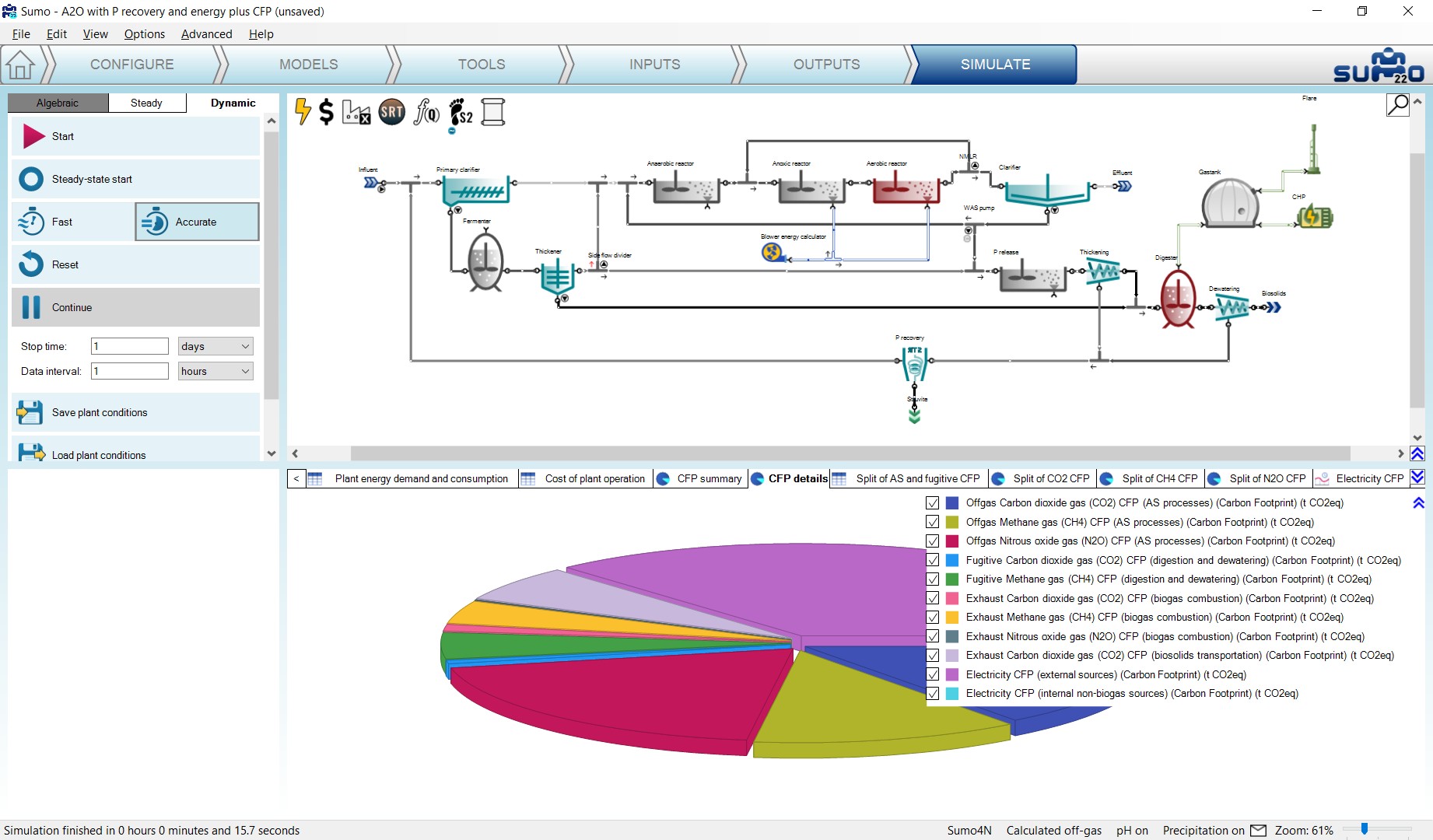
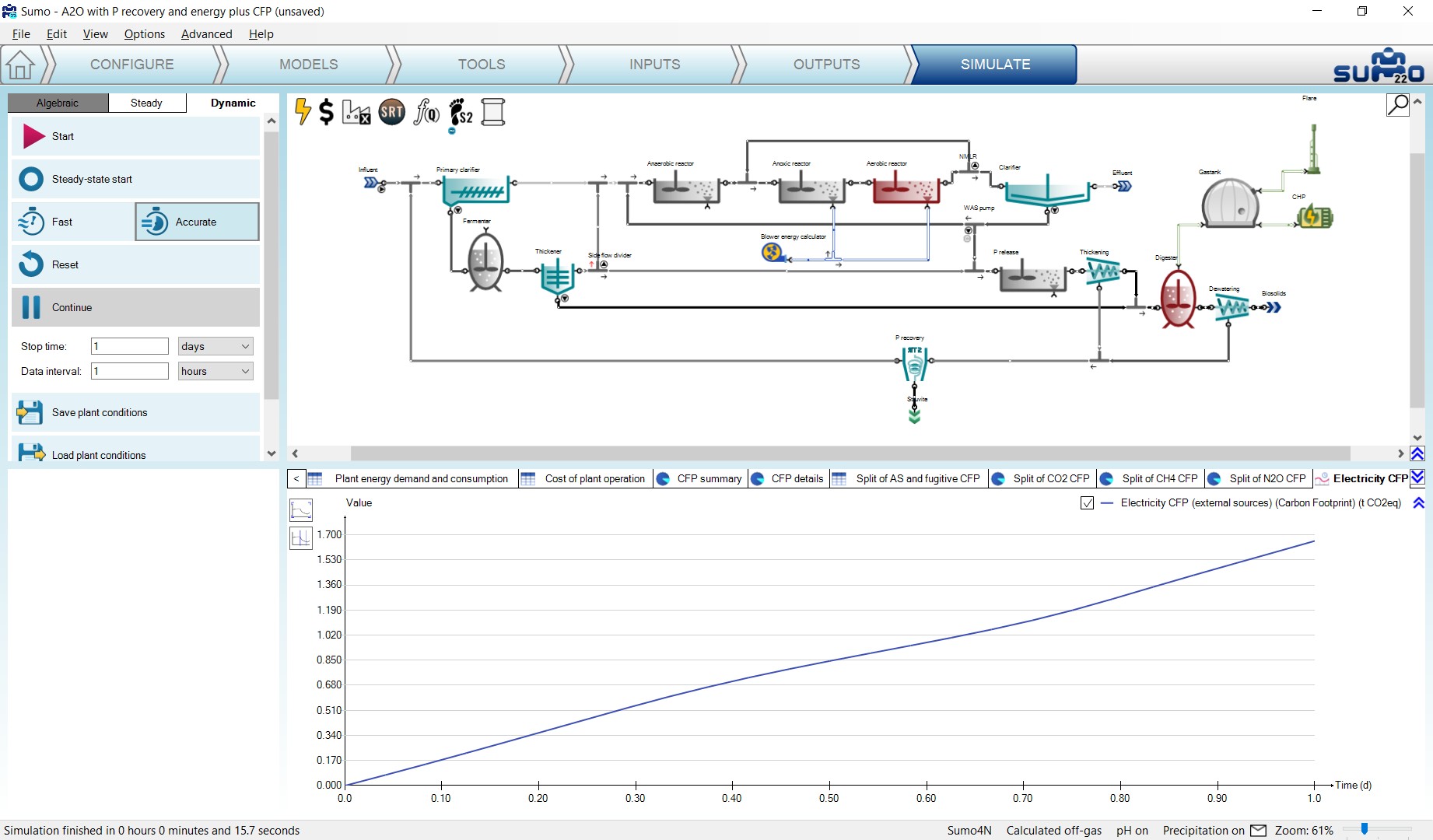
¶ Examples
In this chapter, the built-in example configurations are presented covering various process technologies. These examples can be selected from the Welcome Screen, as well as from the Help menu. They are located in the install directory.
¶ Tutorial plant
This is the example layout used in this manual.

¶ Tutorial plant 2
Tutorial Plant 2 is the extended configuration of Tutorial plant, including mesophilic digestion. Off-gas and pH calculations are turned on.
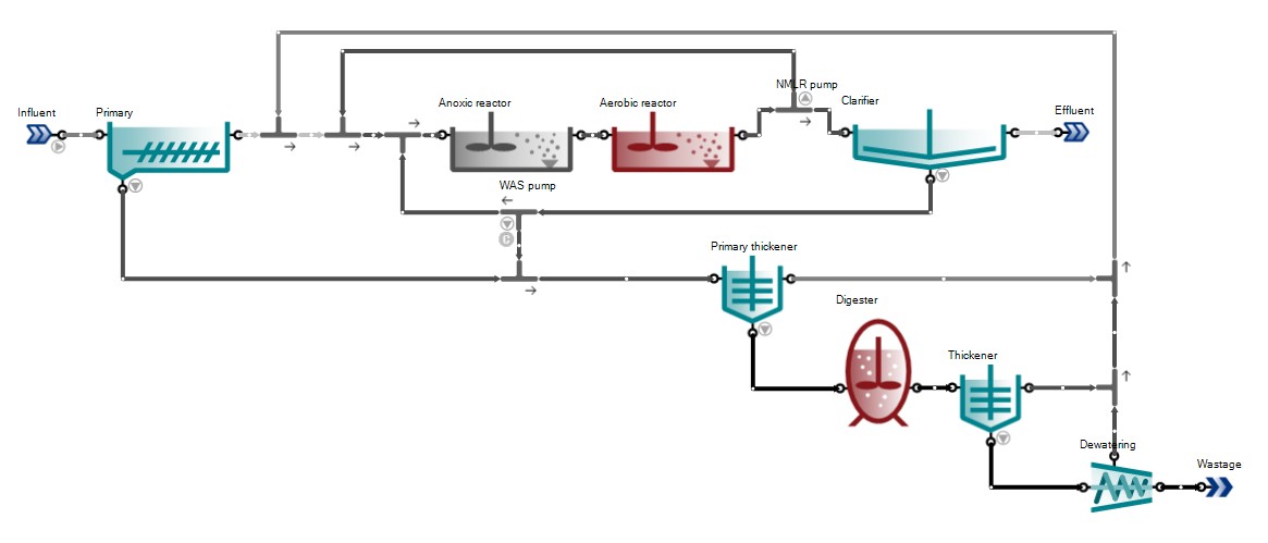
¶ Tutorial plant 2 with energy
Tutorial Plant 2 with energy calculations turned on.
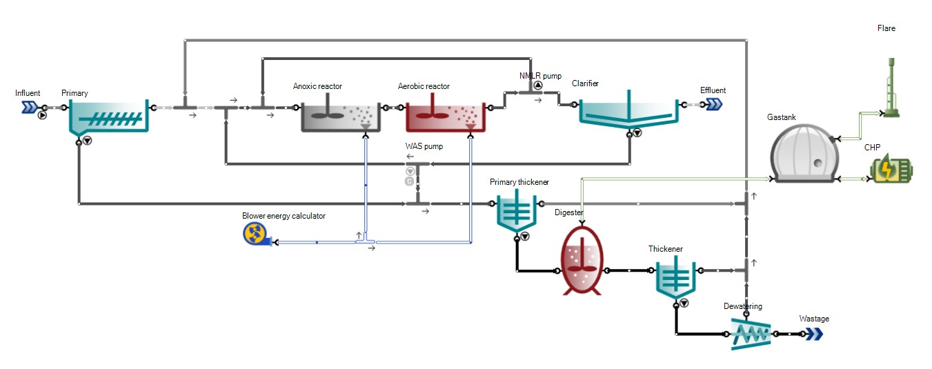
¶ Tutorial plant 3
Tutorial plant 3 is the extended version of Tutorial plant 2 with sidestream treatment (nitritation and denitritation). This configuration is simulated using the two-step nitrification/denitrification model with Sulfur (Sumo2S). Off-gas, pH and precipitation calculations are turned on.

¶ Tutorial plant 4
Tutorial plant 4 is the extended version of Tutorial plant 2 with a different sidestream treatment (partial nitritation and anammox). This configuration is simulated using the two-step nitrification/denitrification model. Off-gas, pH and precipitation calculations are turned on.

¶ A2O plant
A2O configuration with one-step nitrification/denitrification model.

¶ A2O with P recovery and energy
This layout is the extended version of the A2O configuration with primary sludge fermentation, digestion and P recovery (struvite precipitation). Off-gas, pH and precipitation calculations, as well as energy calculations, are turned on.
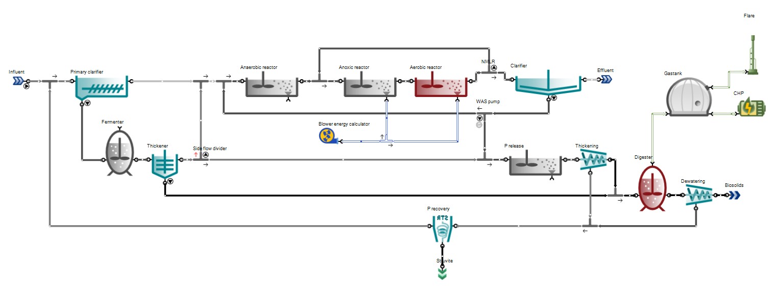
¶ A2O with P recovery and energy plus CFP
This layout is the same as the previous configuration, extended with carbon footprint (CFP) calculations. For the sake of CFP assessment, the underlying process model is changed to Sumo4N in order to improve accounting for nitrous oxide (a very powerful greenhouse gas) production.
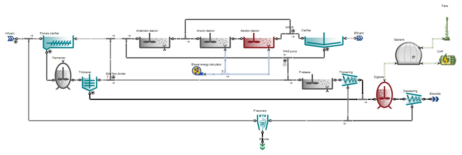
¶ AB plant
This layout features an adsorption/bio-oxidation process configuration, known for enhanced carbon capture.

¶ AB plant with energy
AB plant with energy calculations turned on.

¶ BAF plant
This layout features a treatment plant configuration employing upflow biological aerated filters.
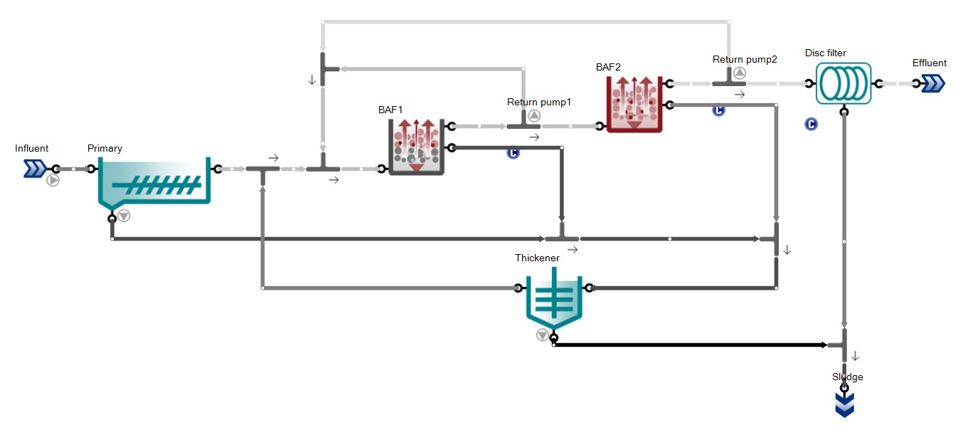
¶ Bardenpho
Five-stage Bardenpho configuration with one-step nitrification/denitrification model.

¶ HPO configuration
This plant demonstrates the application of high purity oxygen to intensify biological wastewater treatment.
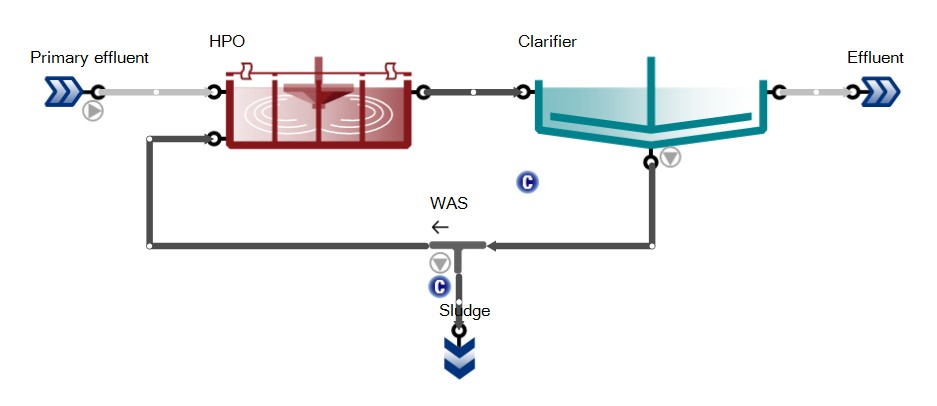
¶ Hydraulic SRT
This plant is a demonstration of hydraulic SRT control. The wastage is removed from the reactor itself, and SRT (irrespective of the MLSS content) will be V/QWAS. Since the reactor volume is 10,000 m3, 3000 m3/d wastage will result in 3.3 d of SRT and loss of nitrification at 12°C.

¶ MLE configuration
Modified Ludzack-Ettinger configuration with one-step nitrification/denitrification.

¶ MLE with energy
This layout is the MLE configuration extended with energy calculations.

¶ MLE with MBR and chemical P removal
This layout is the extended version of the MLE configuration with chemical P removal, using aerated membrane bioreactor as phase separator.

¶ MLE with MBBR
This layout has two parallel MLE trains with wintertime influent to demonstrate the benefits of upgrading the aerobic reactor with media for enhanced N removal.
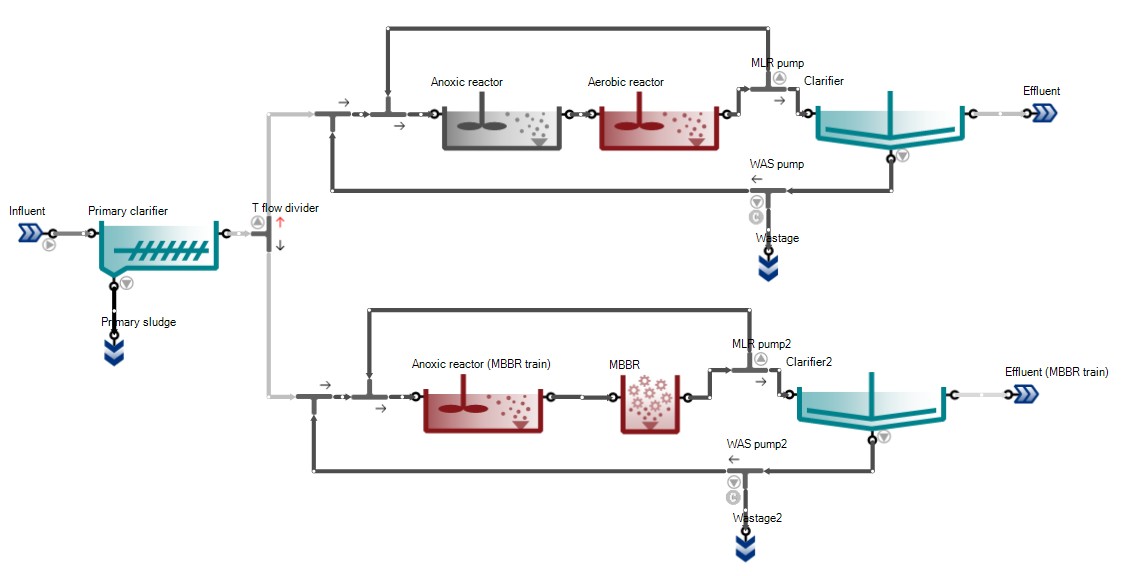
¶ MLE with urban and river catchment extension
This layout is the extended version of the MLE configuration with an urban catchment and simplified sewer system to generate influent loads and a river catchment with river stretches to model effluent impacts on natural water bodies.
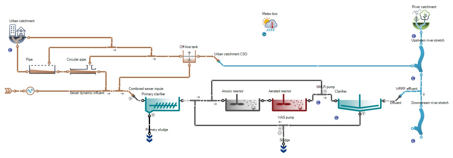
¶ Oxidation ditch
Oxidation ditch example with surface aeration. The ditch is essentially a flow loop and the incoming flow must leave so the outgoing flow must exactly match the influent. The solution to do this in a model is to force the internal flow loop and the rest of the flow overflows to the clarifier. The flow forcing pump does the internal ‘recirculation’ in the oxidation ditch, while the overflow port automatically equals the input flow rate to the ditch.
To calculate the internal flow (which is usually 50-100 times the influent flow) one needs to multiply the forward linear velocity (usually 0.3-0.6 m/s or 1-2 ft/s) in the ditch with the cross sectional area, which will give a m3/d or MGD flow value. This is the value that should be set in the pump.

The Oxidation ditch can be considered ideally mixed as a CSTR for all variables except DO. See the DO profile of the Oxidation ditch on Figure 7.21.
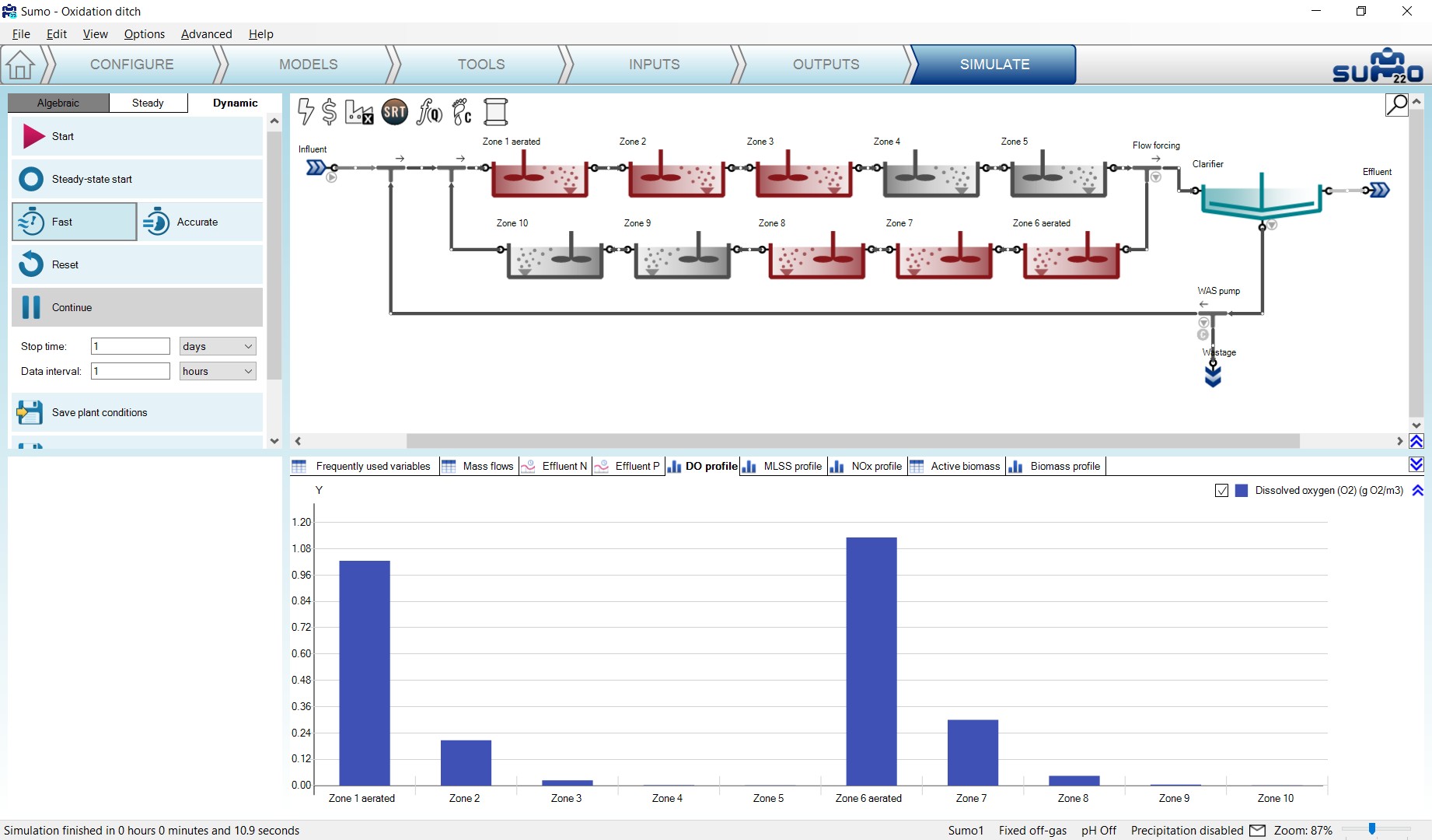
¶ SBR plant
Sequencing batch reactor example with one-step nitrification/denitrification.
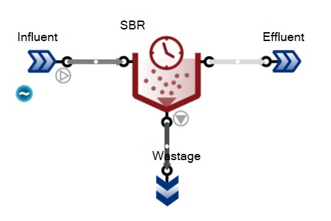
¶ Trickling filter configuration
Simple trickling filter plant example with biofilm model.
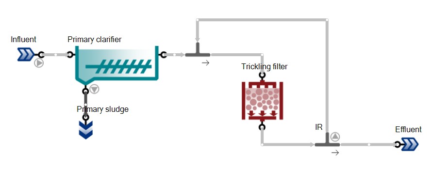
¶ THP plant
UCT plant with THP sludge pretreatment stage before digestion. Off-gas and pH calculations are turned on.
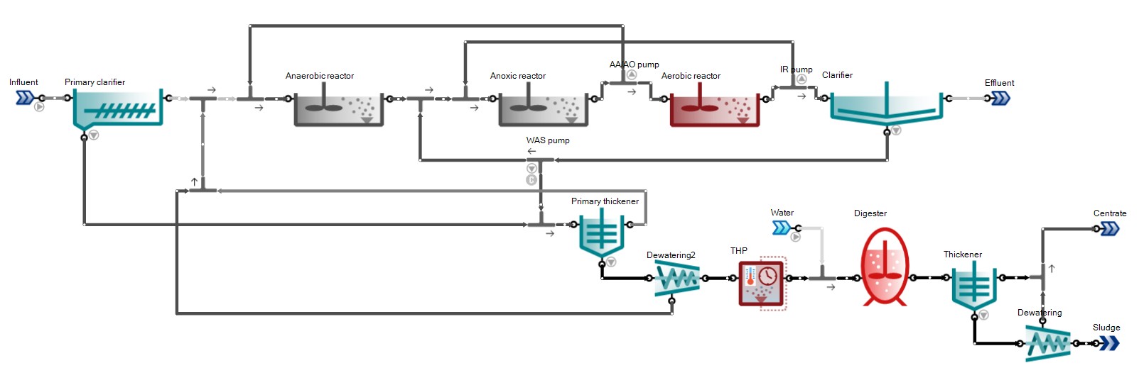
¶ UASB plant with energy
This example layout features a plant with upflow anaerobic sludge blanket reactor with post-aeration and energy calculations turned on.
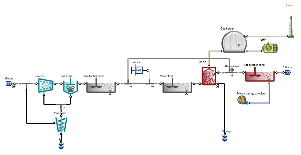
¶ Three lagoons in series
This example demonstrates the long-term behavior of aerated facultative lagoons.

¶ Two ponds with algae
This example demonstrates the long-term behavior of unaerated ponds relying solely on algae and natural surface aeration.
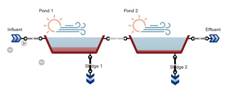
¶ Titration of ammonia solution
This example demonstrates the ammonium/ammonia relationship depending on pH, using an XY diagram, added from the Outputs tab by dropping pH on the X axis and choosing the NH4+ and NH3 in the tank for the Y axis (Figure 7.28).
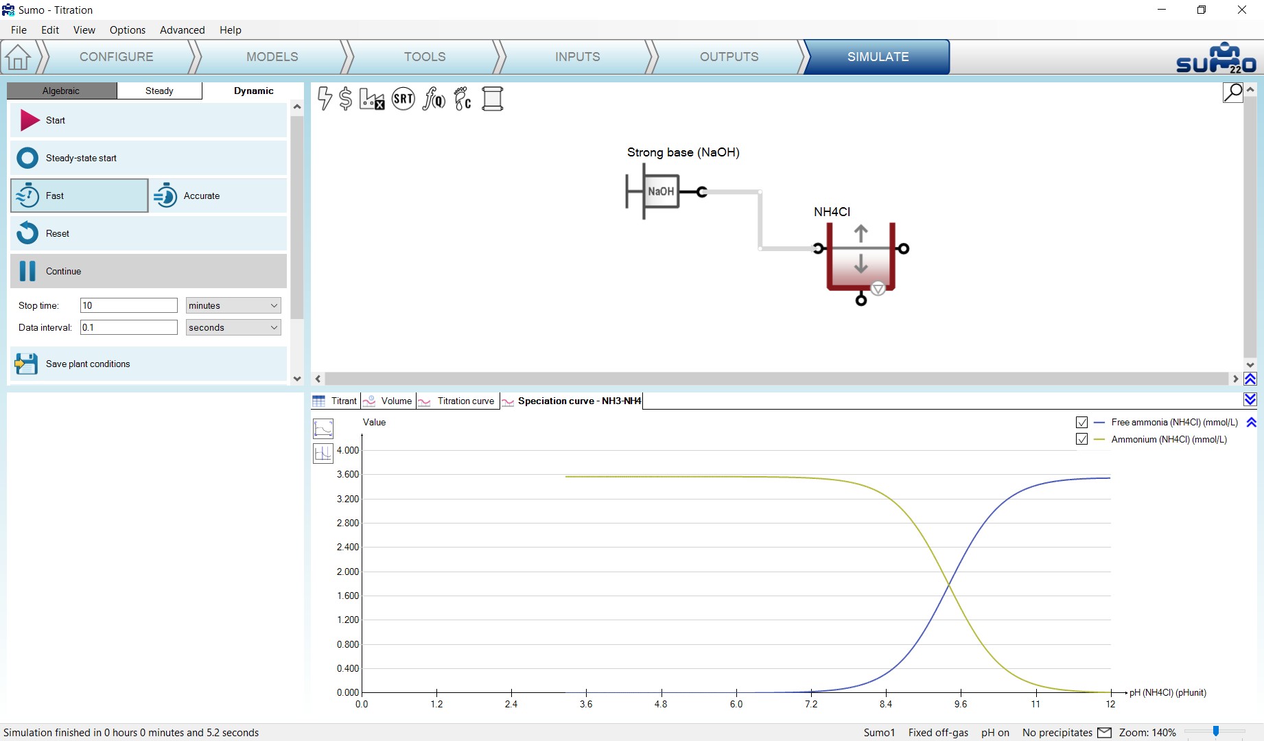
¶ Precipitation
This example demonstrates how the precipitate concentration depends on pH, using the Sumo2S model and an XY diagram, added from the Outputs tab by dropping pH on the X axis and choosing the available precipitates (Calcium carbonate as CaCO3, Amorphous calcium phosphate as ACP, Struvite as STR, Vivianite as Vivi and Iron sulfide as FeS) in the tank for the Y axis (Figure 7.29).
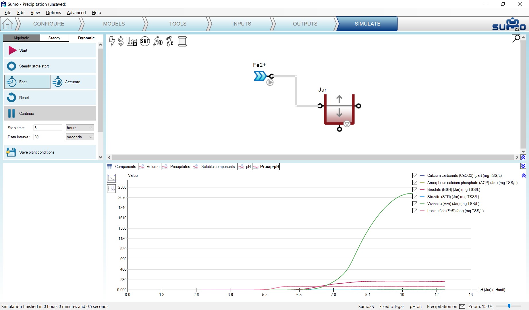
¶ Respirometer
This example demonstrates the possibility of simulating a respirometer (Figure 7.30).
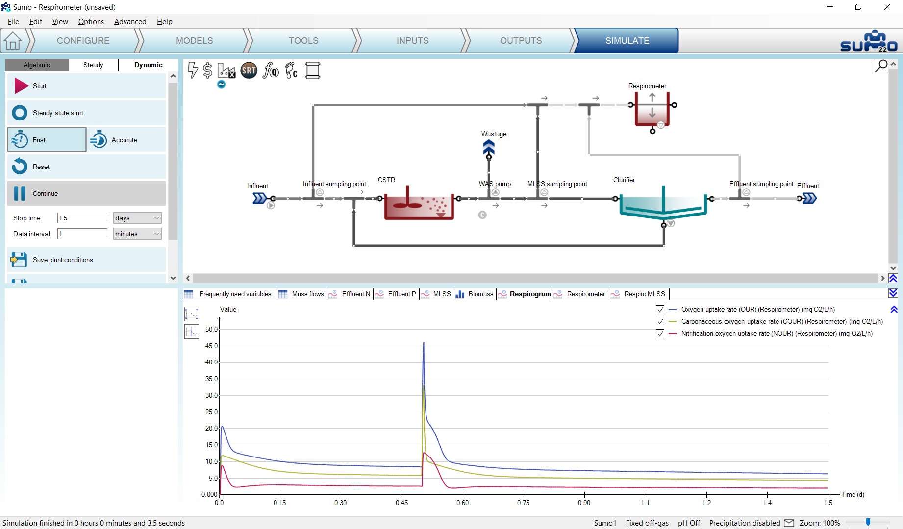
¶ P uptake-release test
This example demonstrates the possibility of simulating a P uptake-release jar test using a sample taken from a plant configuration (Figure 7.31).
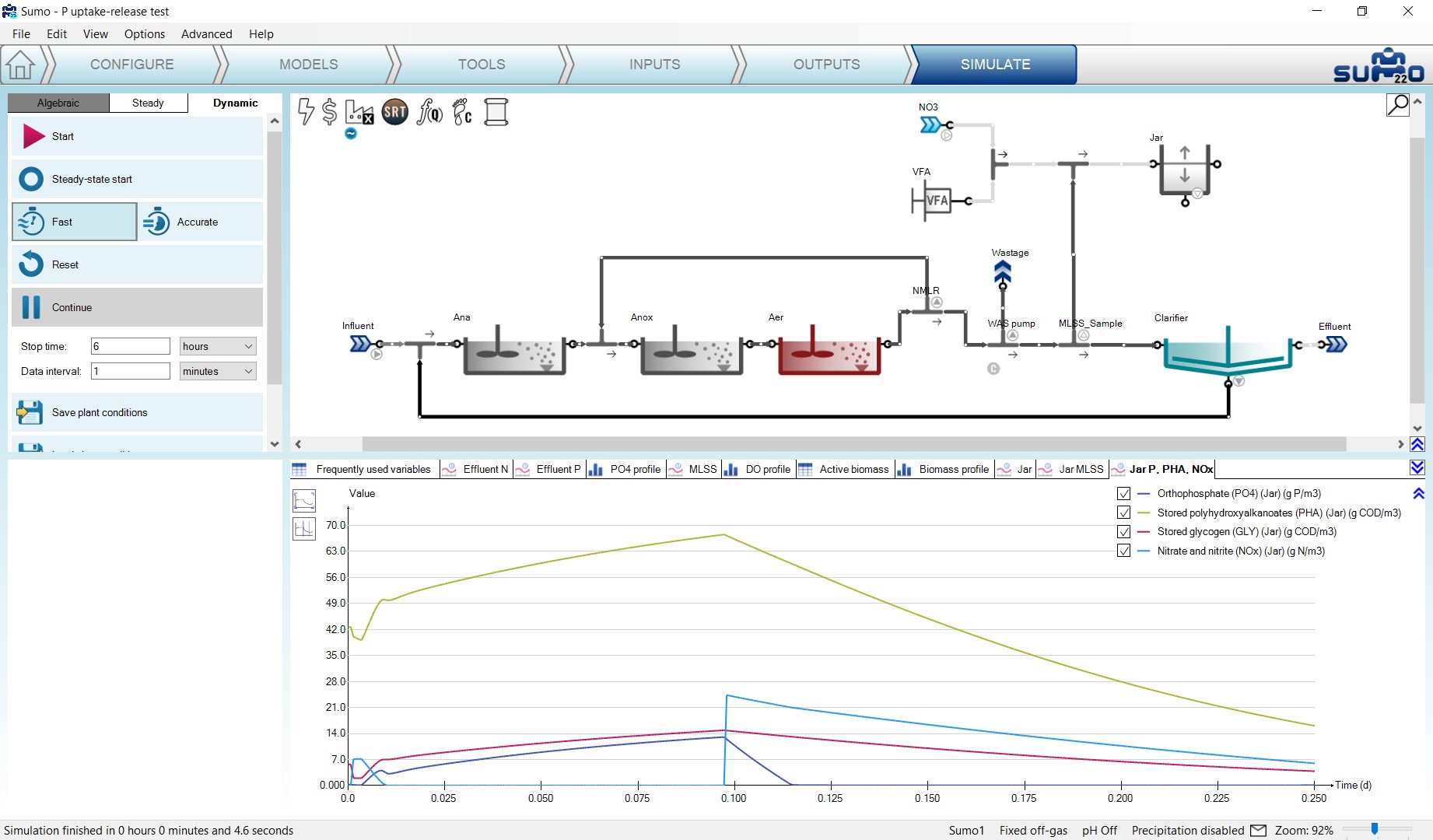
¶ DO and MLSS control
This example demonstrates the implementation of parallel control strategy for MLSS and DO, relying on two PID controllers (Figure 7.32 and Figure 7.33).
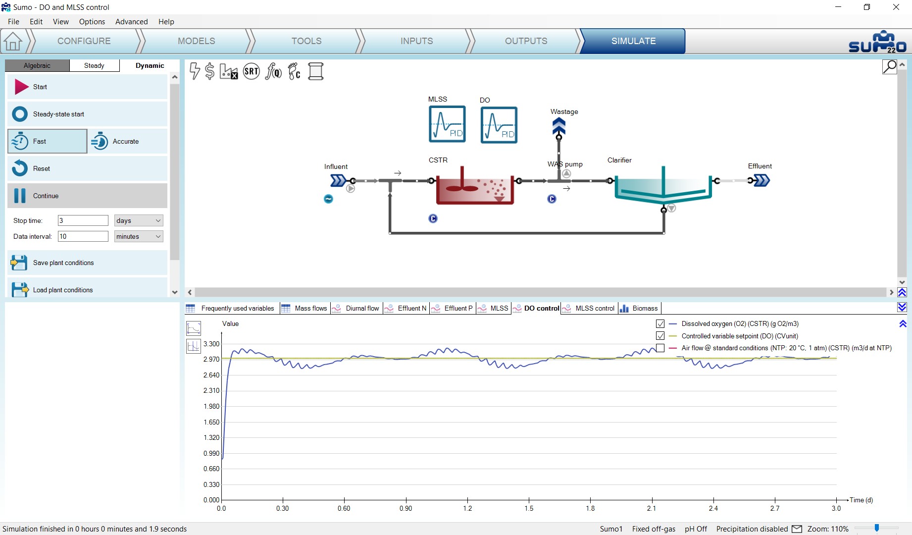
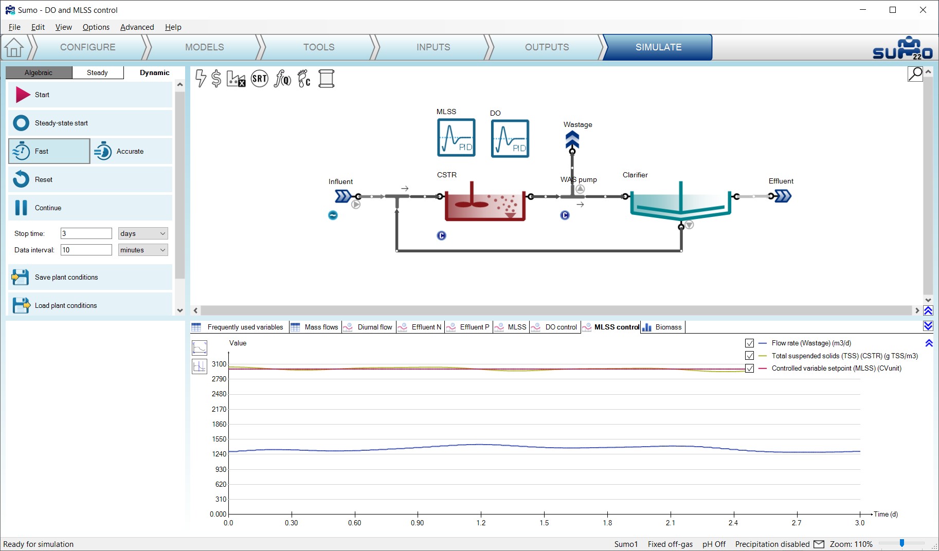
¶ Cascade controller
This example demonstrates the application of the cascade controller strategy for ammonia-based aeration control (ABAC) using two PID controllers (Figure 7.34).
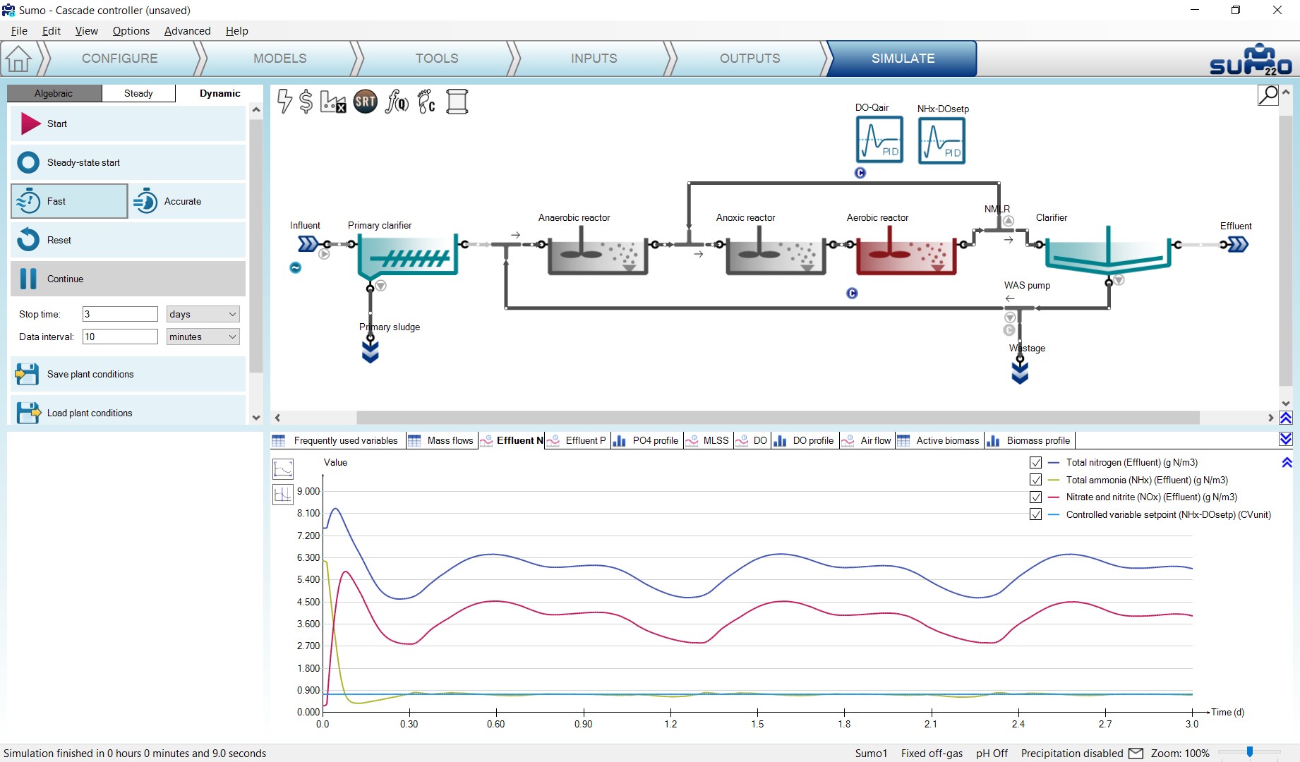
¶ Optimal TN control
This example demonstrates the application of the cascade controller strategy to aerate a reactor according to a setpoint of the sum of effluent ammonia and nitrate concentrations, by using a combination of a PID and a time based on/off controller (Figure 7.35).
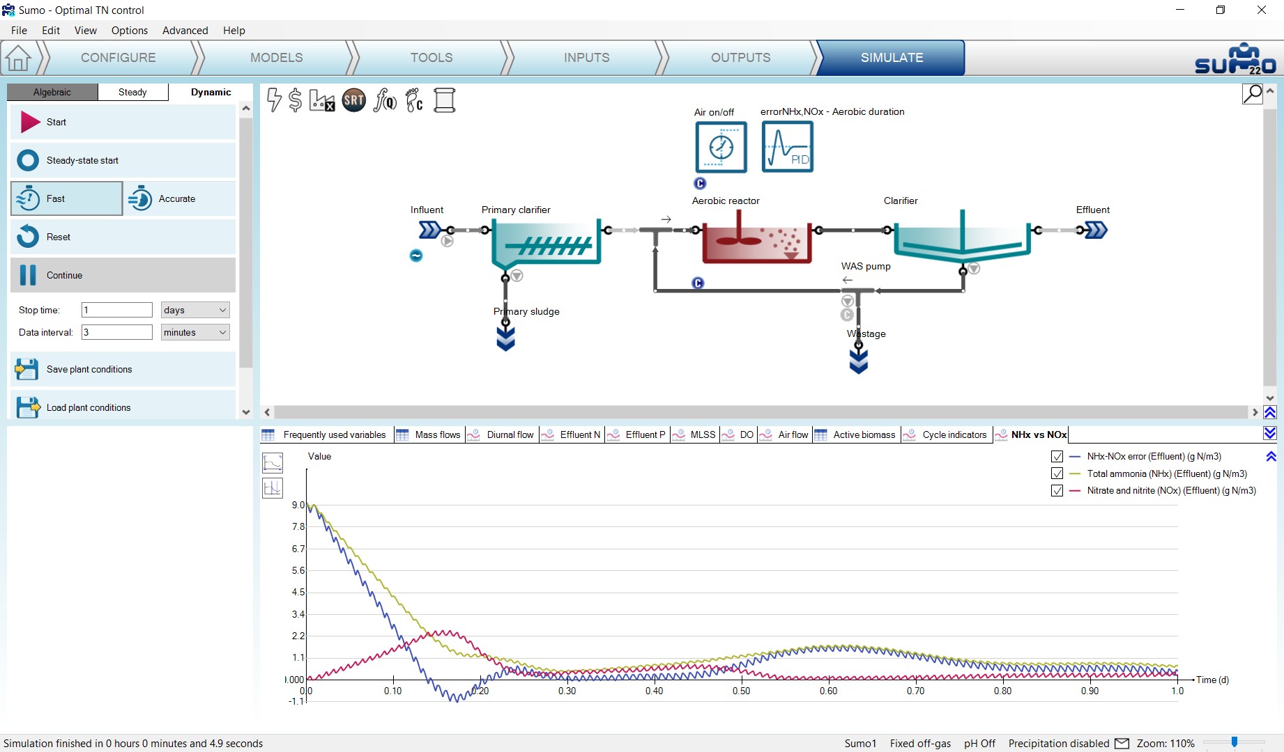
¶ How to use Sumo for plant design
Sumo can be used for plant design as well, based on simple algebraic calculations. This version includes a design tool for AS plants.
AS design calculates the required reactor volume based on design SRT and MLSS.
To set up a plant design example, please follow the steps described below.
¶ Configure
Just like with dynamic configurations, to start the project, the relevant process unit has to be chosen on the Configure tab. For the current exercise, this will be the AS design from the Special units group. This unit is restricted to be only available for the design model. As the selection of the latter will take place in the model setup, at this point the unit will be indicated as invalid, crossed out with red lines (Figure 8.1).
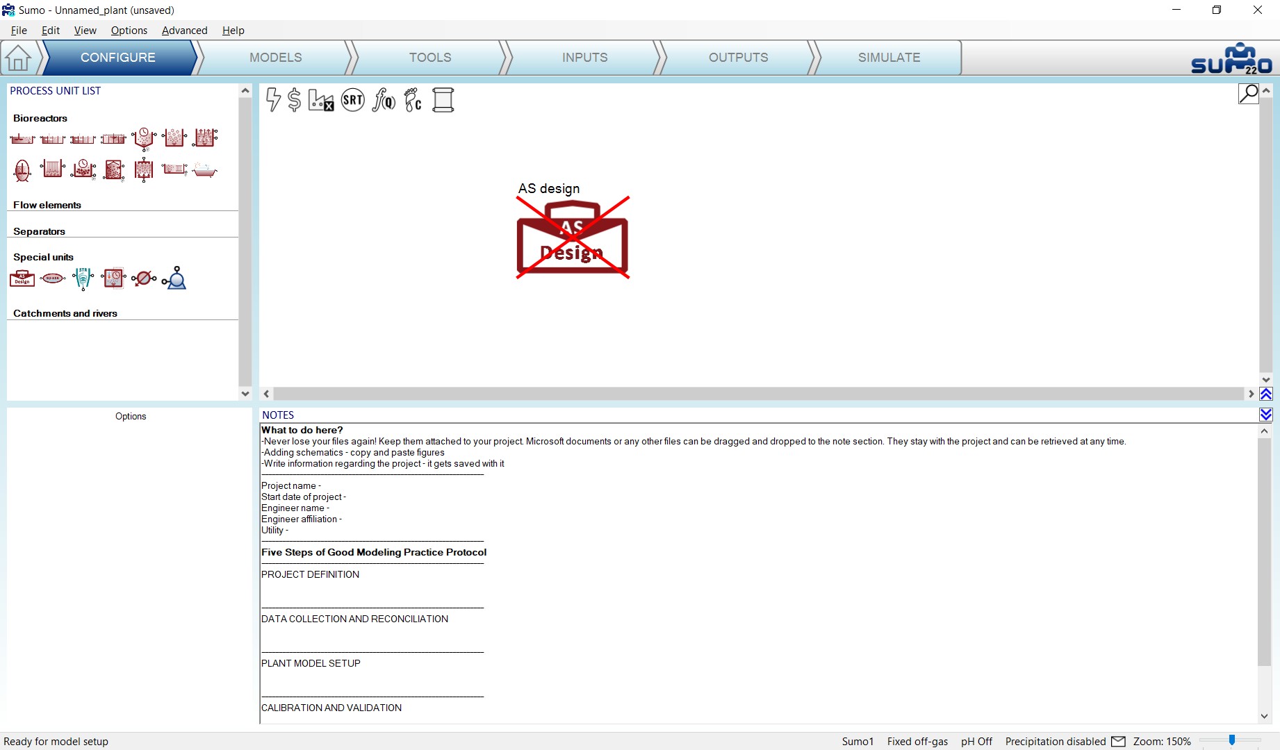
¶ Models
On the Models tab, please choose the Design model on the top left panel, which is available under Model selection/Museum, focus and custom models/Other models/Design. The process unit will become indicated as valid (Figure 8.2).
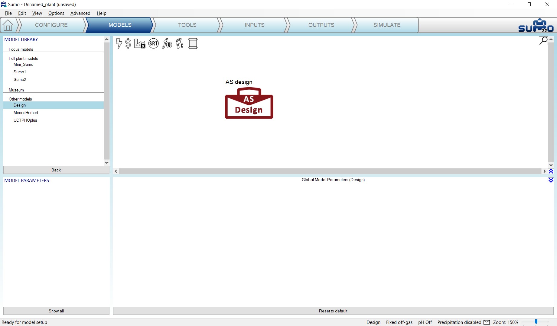
¶ Inputs
On the Inputs tab, the main influent and design parameters can be set (Figure 8.3). By clicking on the Show all button, further details (such as COD and biomass fractions) can be added.
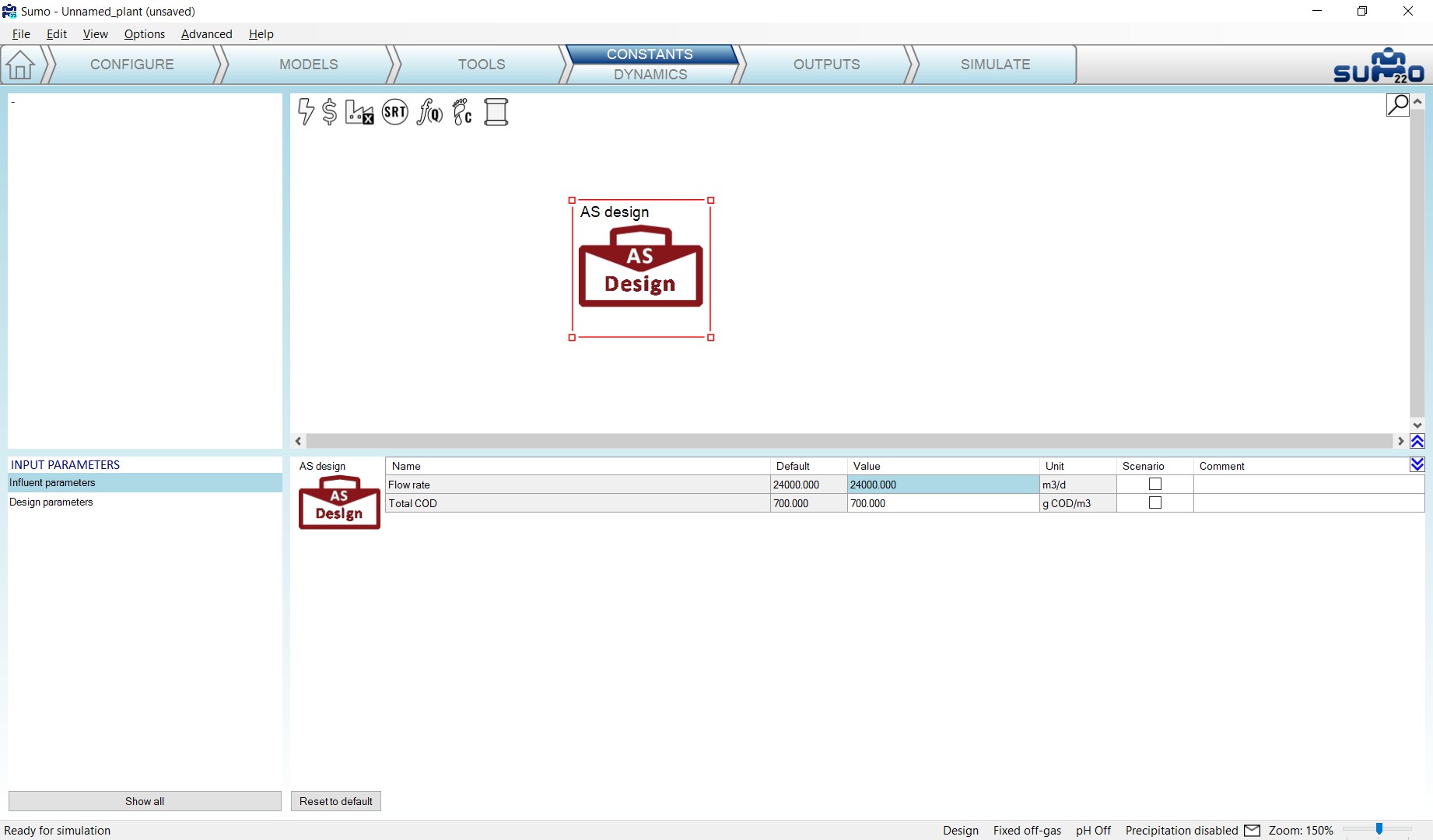
¶ Outputs
Tables can be added here, similarly to the dynamic configurations (Figure 8.4).
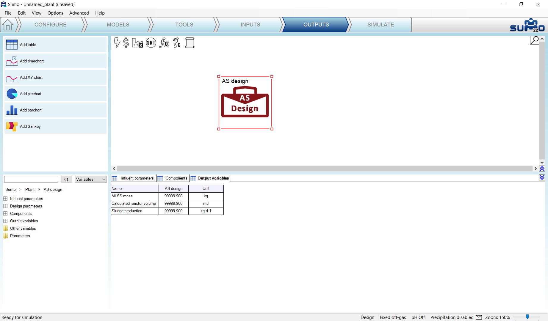
¶ Simulate
On the Simulation tab, the Algebraic mode becomes active. Switching to this tab and clicking Start Algebraic, the desired calculations will be executed and a report can be written of the results. (Figure 8.5)
