¶ Introduction
A model generally can be really complex and at a certain level it is really hard to track where the result came from. There are two different reasons to use debugging tools: the model became unexpectedly slow or the results are not aligned with our understanding and the equations/values behind the scenes needs to be checked.
To check the model simulation speed, a guideline is shared in the first chapter. Walking through the steps might point to the reason of slow simulation.
To help to understand the root of a result and provide some debugging aid Sumo has the XML debugging tool.
¶ Debugging tools for dynamic speed issues
When a SUMO configuration seems to be unreasonably slow, the following commands may provide information on the reason.
¶ User Script
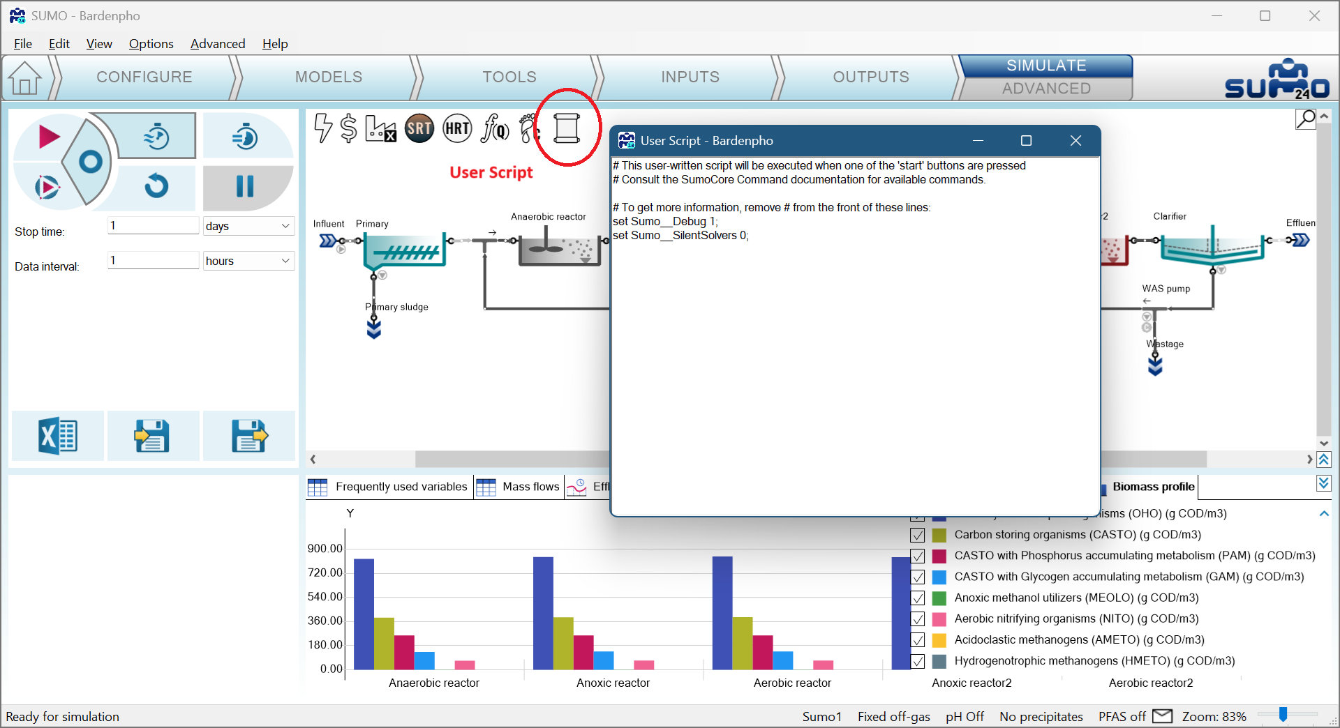
Activate at the User Script debug features by removing the # from the following commands. To edit the User Script click the note icon on the top of the drawing board or got Advanced|Usersript menu:
set Sumo__Debug 1; # enables more debug messages
set Sumo__SilentSolvers 0; # Switches solver related error messages on
Note
- “#” means comment
- The User Script is automatically saved with the configuration, and executed at every Start.
- Messages show up in the mail icon on the bottom right.
¶ Main reasons
The main reasons for a slow run are:
- Incorrect input specification (e.g. tiny reactor volumes, incorrect ion specification)
- Very large configurations
- Many loops, recycles, etc. Particularly complex loops without reactors
- Separators where the desired solids are specified, not the flow
- Slow computer
- Potential code problem
¶ Gather information
To collect background infromation from the simulation engine, the source code of the model is available from the XML debugger (see next chapter how to use it). There are key variables to look at as a first step after a run.
¶ Key variables
The next step is to create a table at OUTPUTS tab:
- Switch to Raw search on the bottom left panel
- At the middle left text bar search for
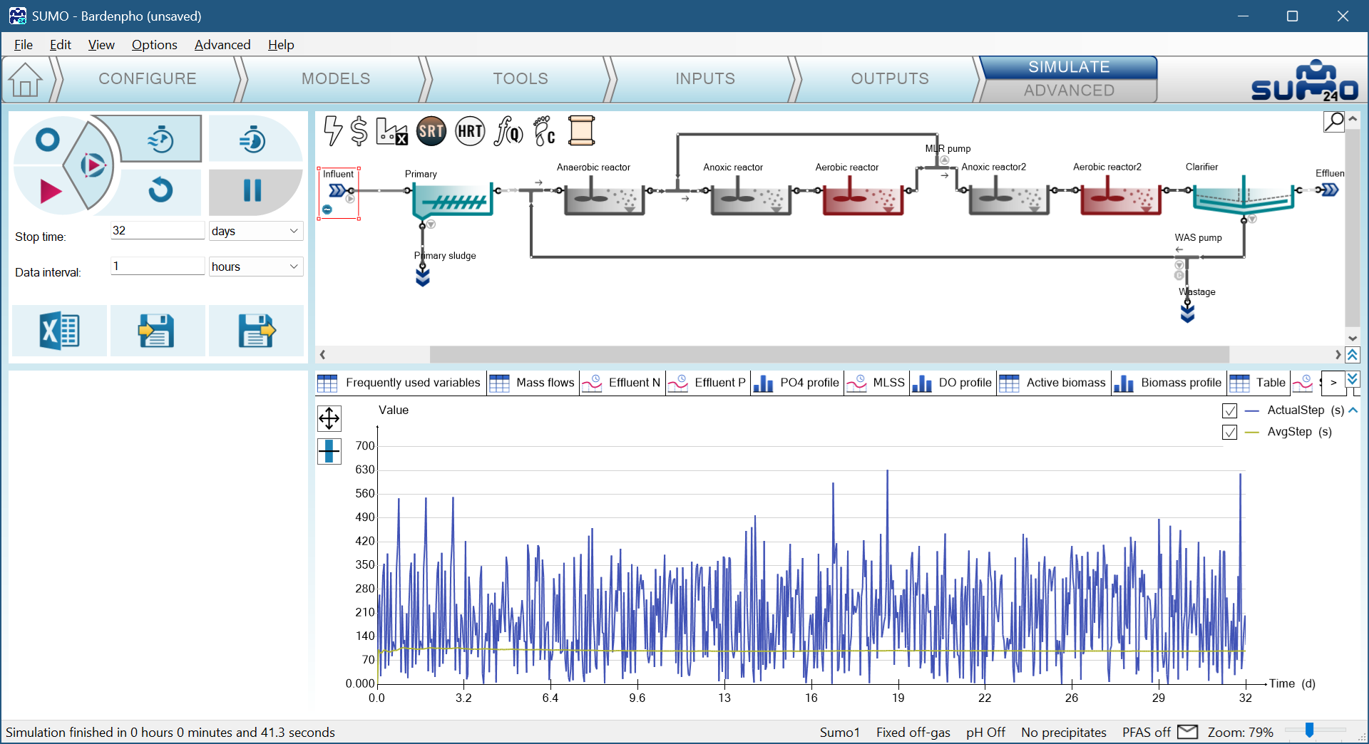
- ActualStep: time between the last two steps (constrained by Data interval)
- AvgStep: average stepsize during the simulation
- MaxAbsDerName: Symbol of the derivative with largest value at the last step
- MaxAbsDerSigned: Signed value of the largest derivative at the last step
- SystemSize: number of states in the model
and drag them to the table.
- Look for loop errors (i.e. for flow loop errors type Q_error, for aeration loop errors SSOTE_error) and drag them to the table.
- There might be other loops with TSS or state variables in the model. The residual error at every timestep should be a small number, less than 1e-8 if the loop is solved.
The table in the Bardenpho example after 100 days looks like this:
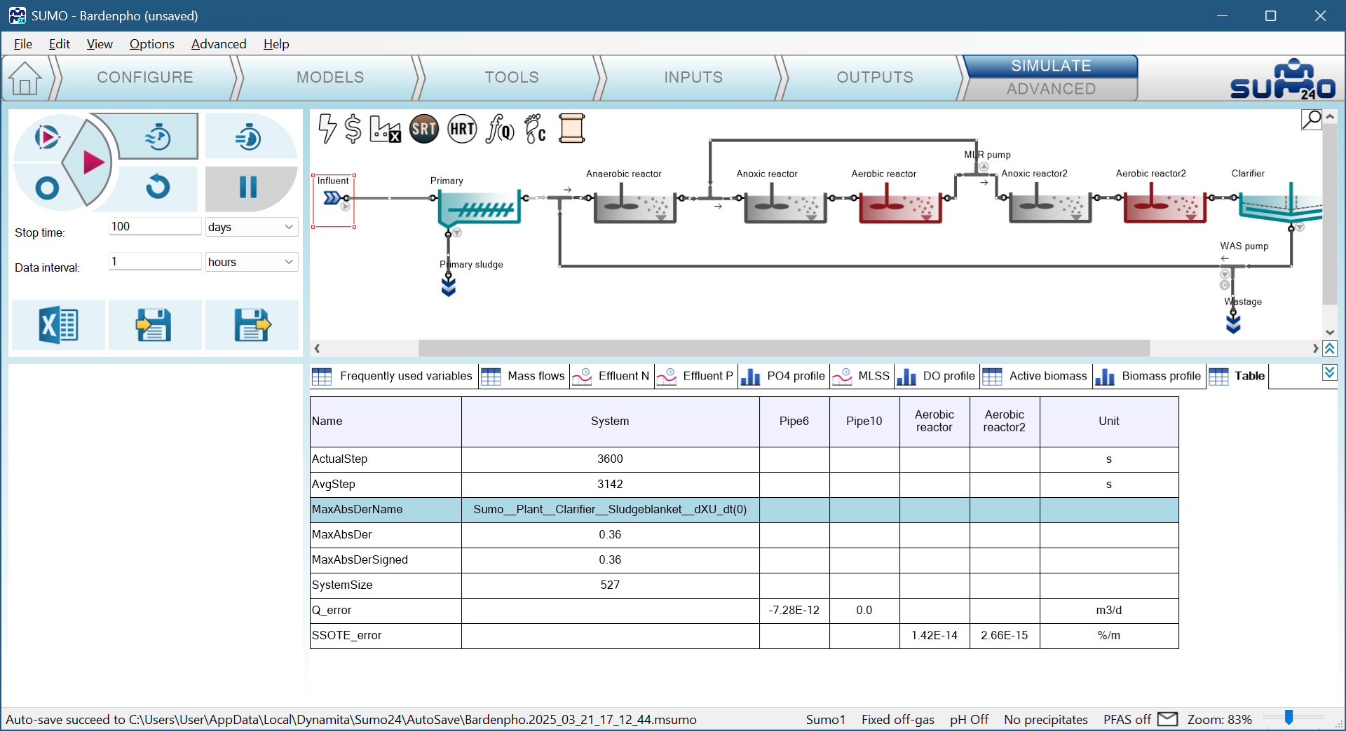
This table shows that the highest derivative was the XU concentration (unbiodegradable particulate COD) in the sludge blanket. If the model runs normally, it does not get stuck on one variable, but switches between them as it progresses. You can also put _error variables on timecharts to see them dynamically.
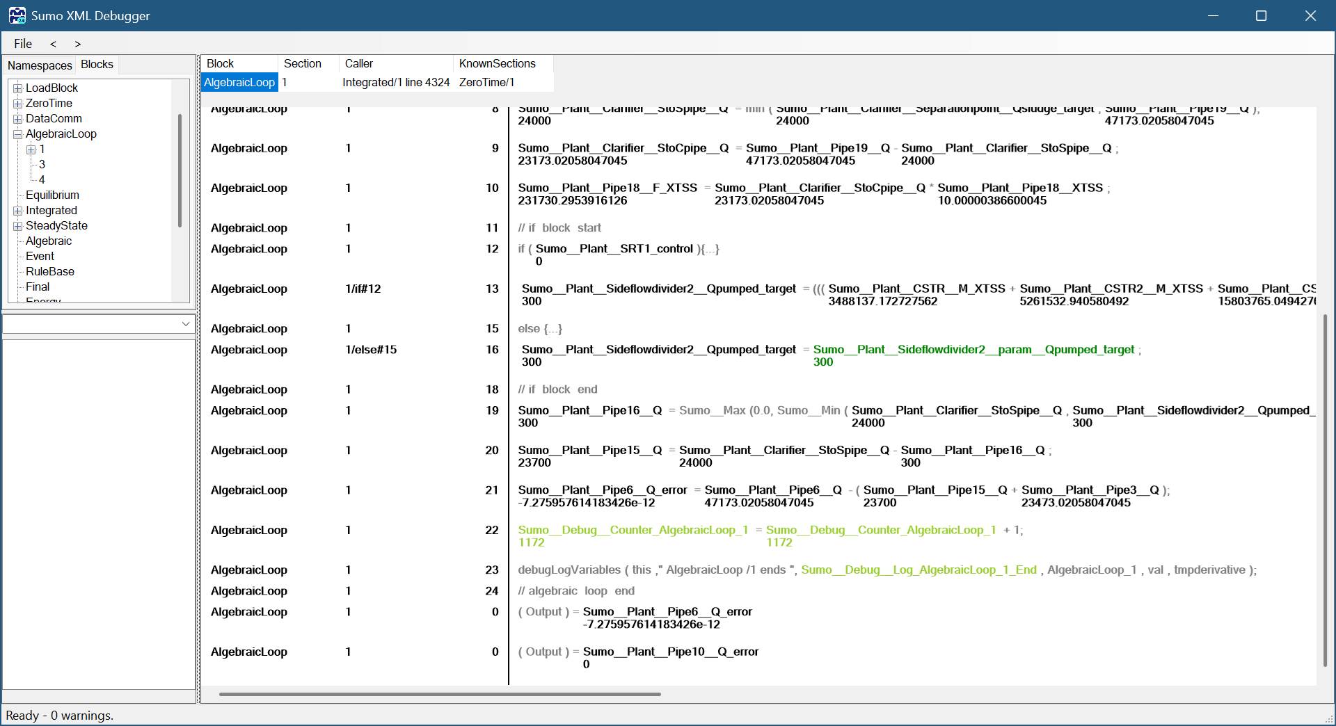
Another approach to check the loop errors is at the XML debugger's Blocks tab, check the “AlgebraicLoop” block. At the end of each blocksection, you will find one or more variables ending with _error, such as Sumo__Plant__Pipe6_Q_error and Sumo__Plant__Pipe10_Q_error:
¶ Steps
It is useful to put ActualStep, AvgStep on a timechart. In most cases the steps start out small then quickly increase to the value of the Data Interval (default: 1 hr, 3600 sec). It is normal to see reduced steps even during a run without any changes.
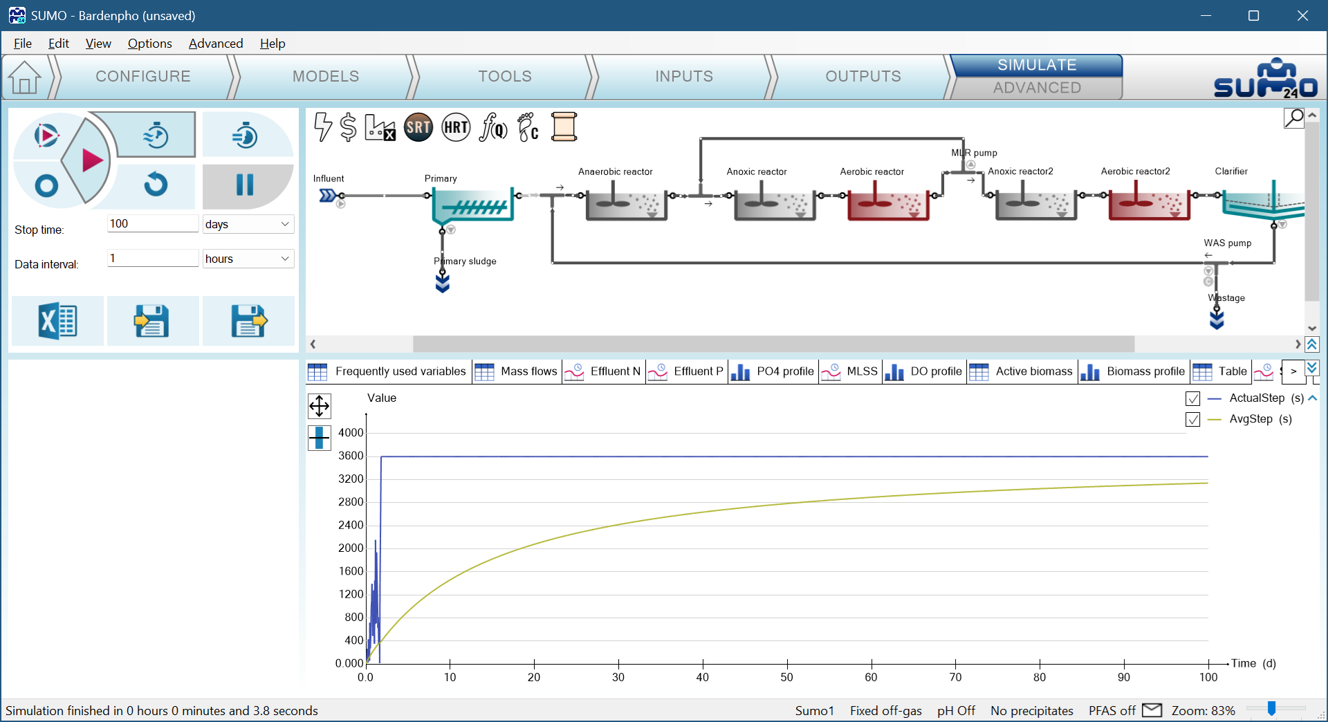
Dynamic influent, or other dynamic data will always reduce the timestep. Interpolation between dynamic datapoints will slow down the solver significantly. The next image shows the birthday cake added to the influent, compare the stepsize to previous run.
This procedure may point to the problem reactor or variable which then requires closer investigation.
¶ Counters
An additional layer of information about speed can be collected by following the counter of different evaluations. These counters can be added to a table at the OUTPUT setup with the Raw filter by opening the Debug block:
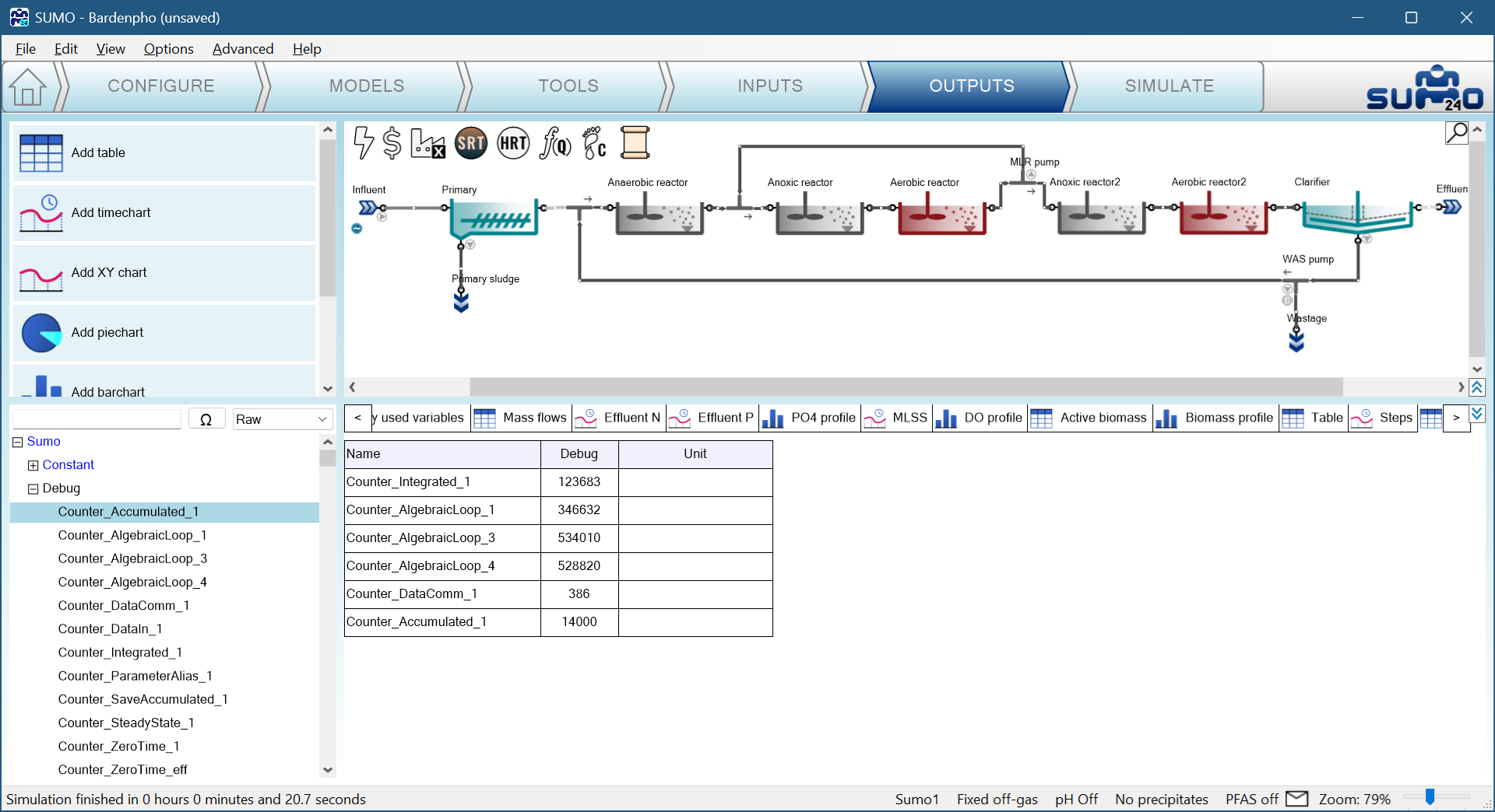
The integrated counter shows the number of integrated block evaluations, the algebraic loop the loop evaluations, the DataComm refers to the number of Data Intervals during the simulation and the Accumulated shows the number of steps (StopTime divided by this gives the Average step of previous steps). The information collected from these numbers is the following: What is the Loop per Integrated counter ratio? If the ratio is higher than 5, it will mean that the algebraic loop is tricky to solve and will take a lot of time to find the right solution.
If the pH calculation is on, similar counters are available for the Equilibrium calculations where the Equilibrium to Integrated ratio is important above 15 the pH solver is struggling and results in slow run.
¶ XML debugger: How to open and load a model
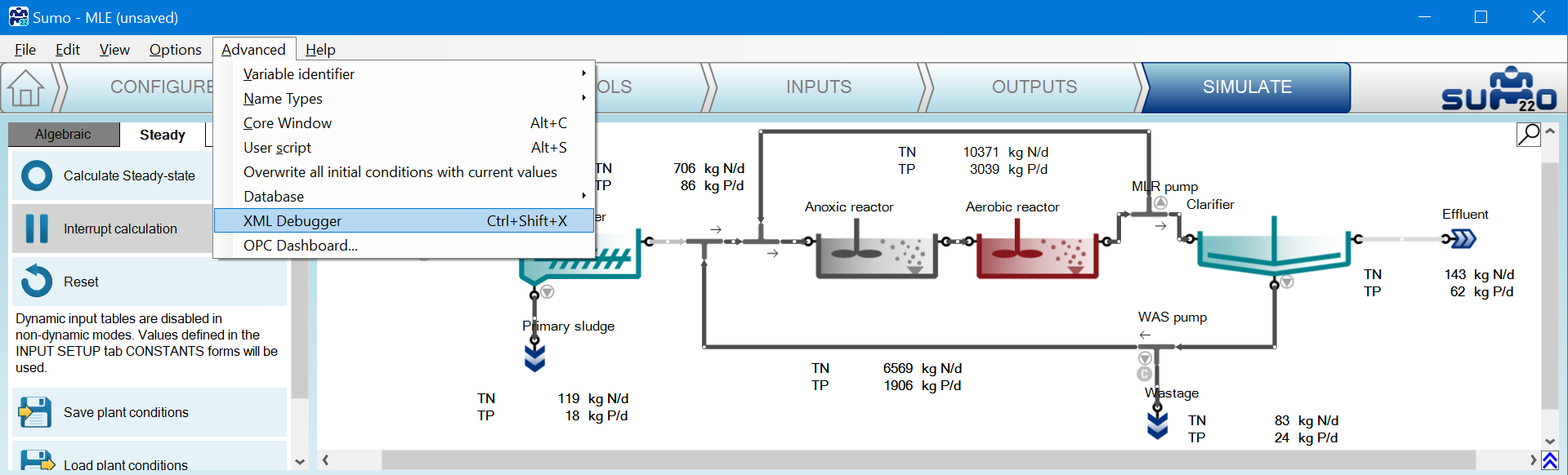
When the model doesn't predict the numbers it should, it's usually a good idea to check its inner workings and see how things are calculated. The XML Debugger lets you do this in a simple way. We will use the MLE plant as an example, how to use this tool.
¶ Start XML debugger
Once you've run the simulation to the state that you want to debug, click XML Debugger in the Advanced menu, or press Ctrl-Shift-X:
- A new window will be opened called Sumo XML debugger:
- Load the xml of current project:
- Click File → Load Current XML, which will load the code behind the currently running model:
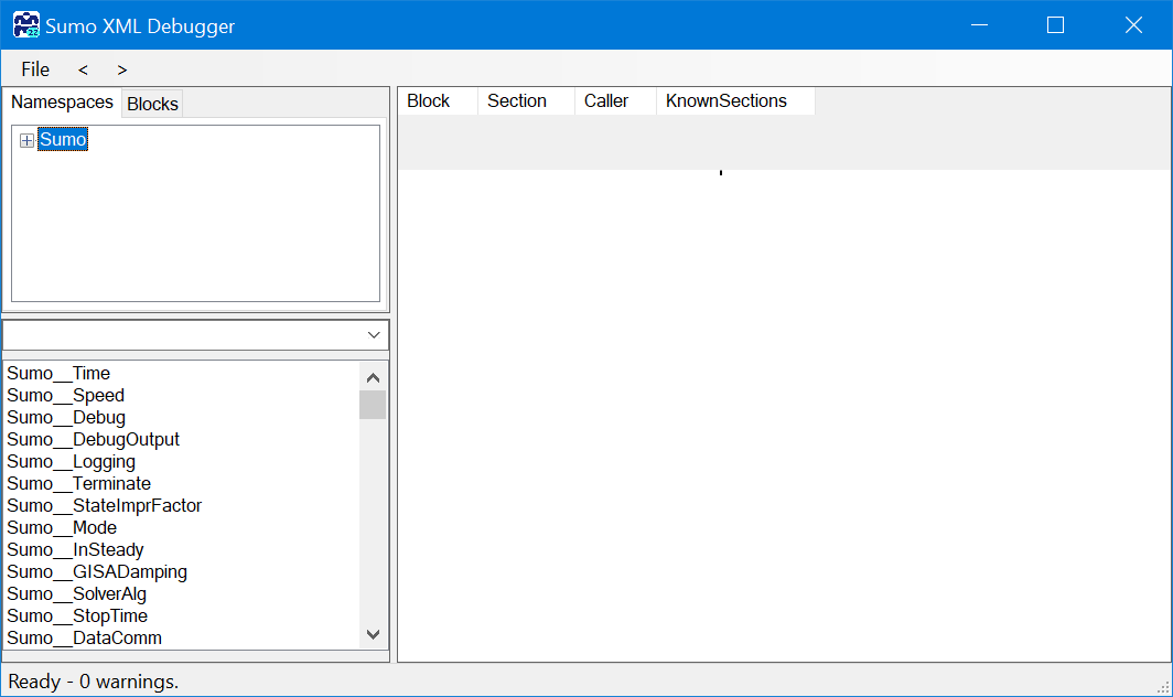
On the left hand side there are three blocks:
- Namespaces and Blocks tabs:
- Under Namespaces the structure is identical to the setup seen in the Advanced CoreWindow and similar to Output setup bottom left panel with Raw settings). each layer is considered as a namespace and build up the Incode name of the variable (short description about these can be found in the Plantwide excel calculation chapter).
- Under Block the structure is following the model structure differently. In this part you can follow the order of calculation blocks, as loading functions, parameters, initializing variables at ZeroTime, calculations in DataComm or the structure of Algebraic loops in the model.
- search field and
- list of variables based on search field and namespace selection.
You have the option to load and browse other XMLs or even build some, but you will only get the numbers for the current one.
¶ Find variables
Once the xml is loaded the blocks can be opened and variables can be selected from the left side of the window (maximize window can help to see everything).
In this example we will check why the Primary sludge flow is different from the expected, thus start at the sludge flow: understand how the primary sludge flow is calculated.
¶ How to: find the variable symbol for check
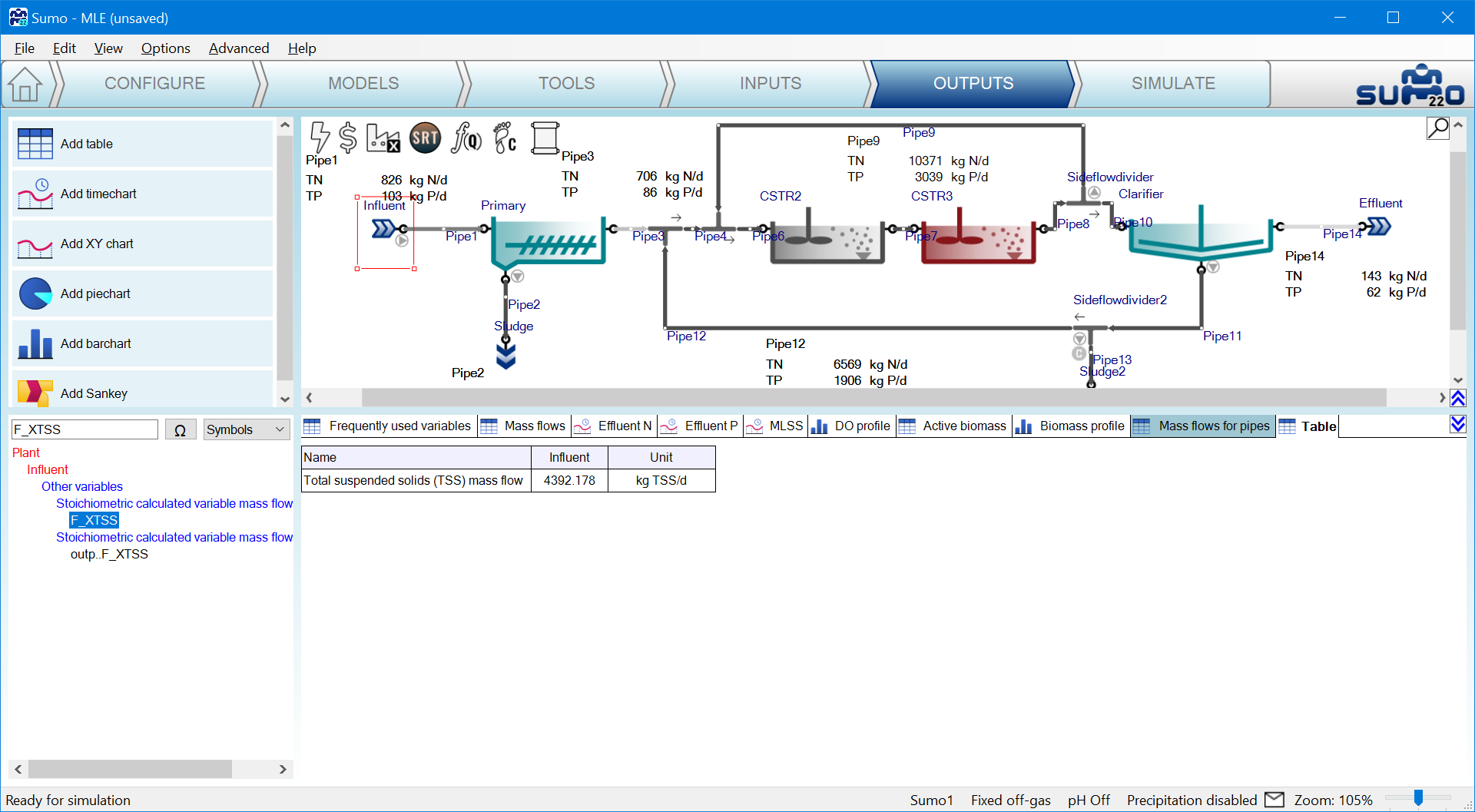
There are various ways to find the symbol of the variable we want to follow in the debugger. The easiest one is to start from Sumo Outputs tab. Go to the opened Sumo project Outputs tab and change the:
- Advanced|Variable identifier to Symbols
This will change the Name column in any input or output table to Symbols and will show the relevant symbols. - Advanced|Name types to Incode names
This will change the displayed names of process units on the drawing board and in any table header or chart legend. The setting helps to navigate through the debugger plant structure.
Let us see how this translates for the primary sludge flow. On the figure below (XML Figure 4) the unit names changed as well as the variable names in the table first column. The Mass flows table starts with symbol 'Q' which originally showed up as ‘Flow rate’ (Advanced|Variable identifier|Name). However the column headers are numbered pipes and not unit names as we are looking for. By switching on the View|Show pipe names option we could identify the primary sludge pipe or simply drag and drop the Sludge unit to the table. You can move the column next to Pipe2 and see they have identical values.
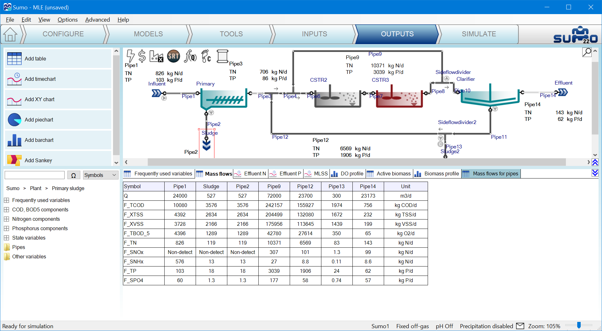
The variable symbol of the primary sludge flow rate is ‘Q’ of the Sludge unit in this project.
¶ Search for it in the debugger
After identifying the symbol of the variable there are various ways to find the variable.
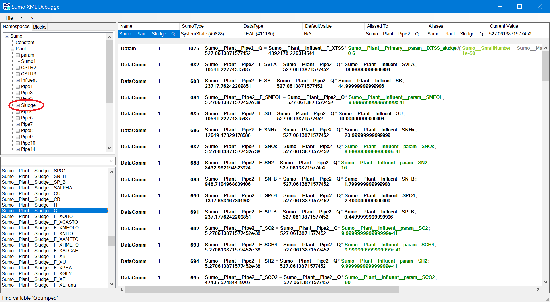
¶ The structure of Namespaces
Go directly to the Namespaces: Sumo|Plant|Sludge. It will list at the bottom all the variables used in the Sludge process unit. The list is extensive but the ‘Q’ is there.
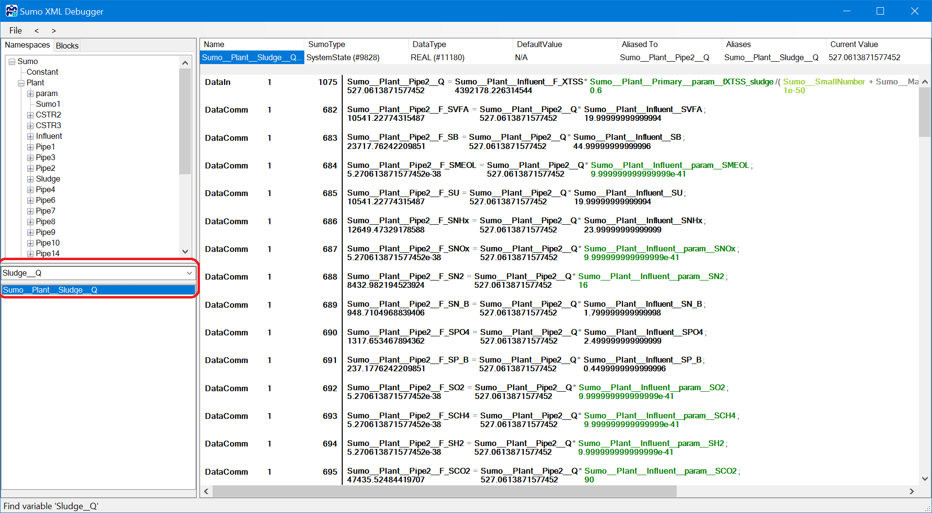
¶ Search
Type in the variable symbol as a general convention: unit name__variable name so in this case Sludge__Q.
The full Incode name of the variable does not contain any special characters and the namespace levels are separated by ‘__’ every time. The search field accepts regular expressions to easier control the list of results.
¶ Check variable calculation
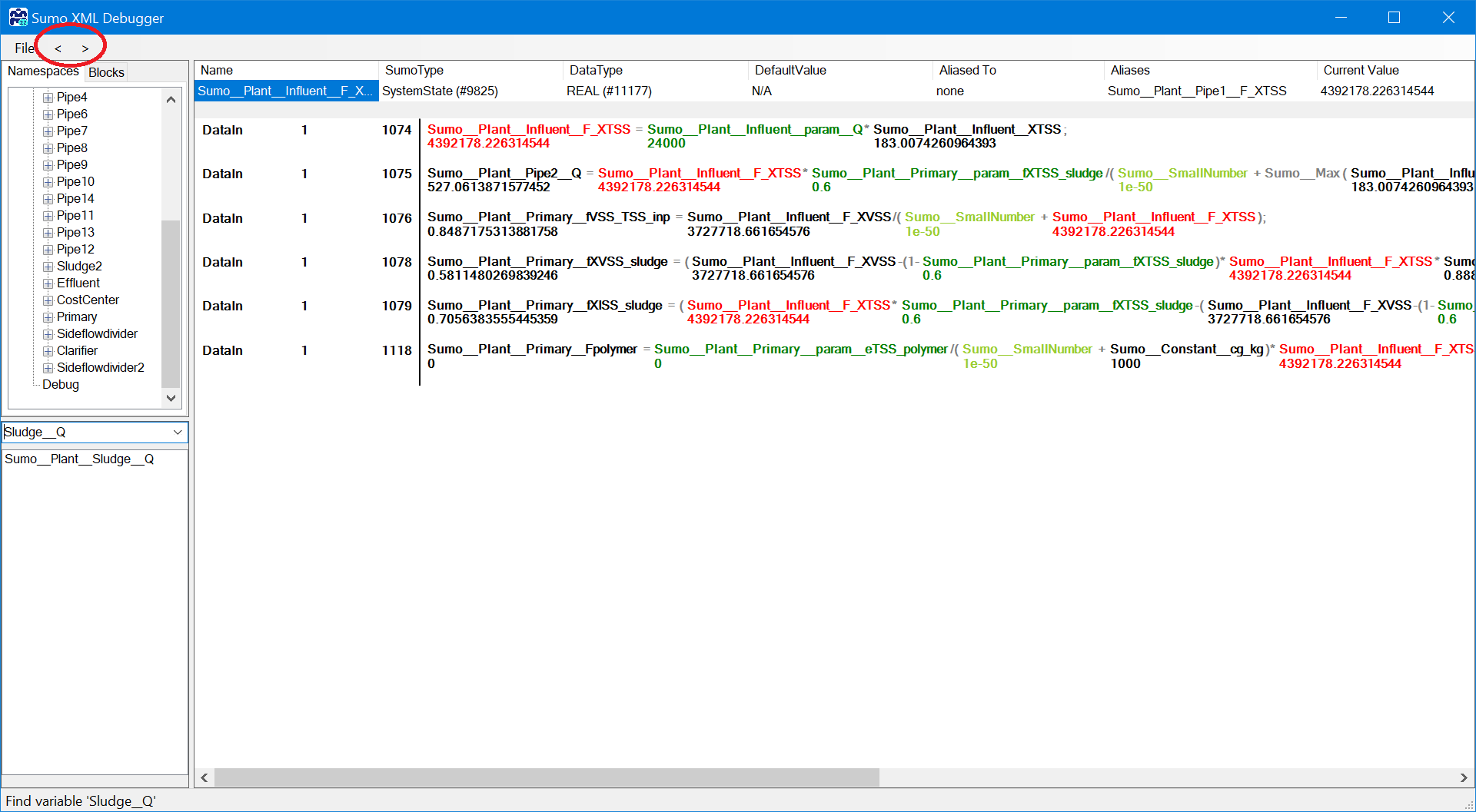
Once the variable is on the list at the bottom left panel, select it. On the right hand side the following information is available:
¶ Variable specification
The top section shows the variable specification:
- Name: full incode name of variable
- SumoType: Parameter, Constant, StateVariable, Systemstate (any calculated variable), etc.
- DataType: Real, Integer, Boolean, Array, etc.
- DefaultValue: default value for parameters
- Aliased to: The linked variable with identical calculation logic, this the value of this variable and the 'Aliased to' variable always will be identical
- Aliases: the list of aliased variables connected to the variable indicated at 'Aliased to'
- Current value: the latest calculated value of the variable in Sumo (only available if the current XML is loaded)
¶ Calculation of the variable
The first row below the specification is always the equation how the variable is calculated: left side is the variable and right side is the expression. It starts with the codelocation (when the calculation is performed, for details see the Book of SumoSlang), blocksection, row and it ends with the equation as below (you have to scroll to the right to see the full equation):
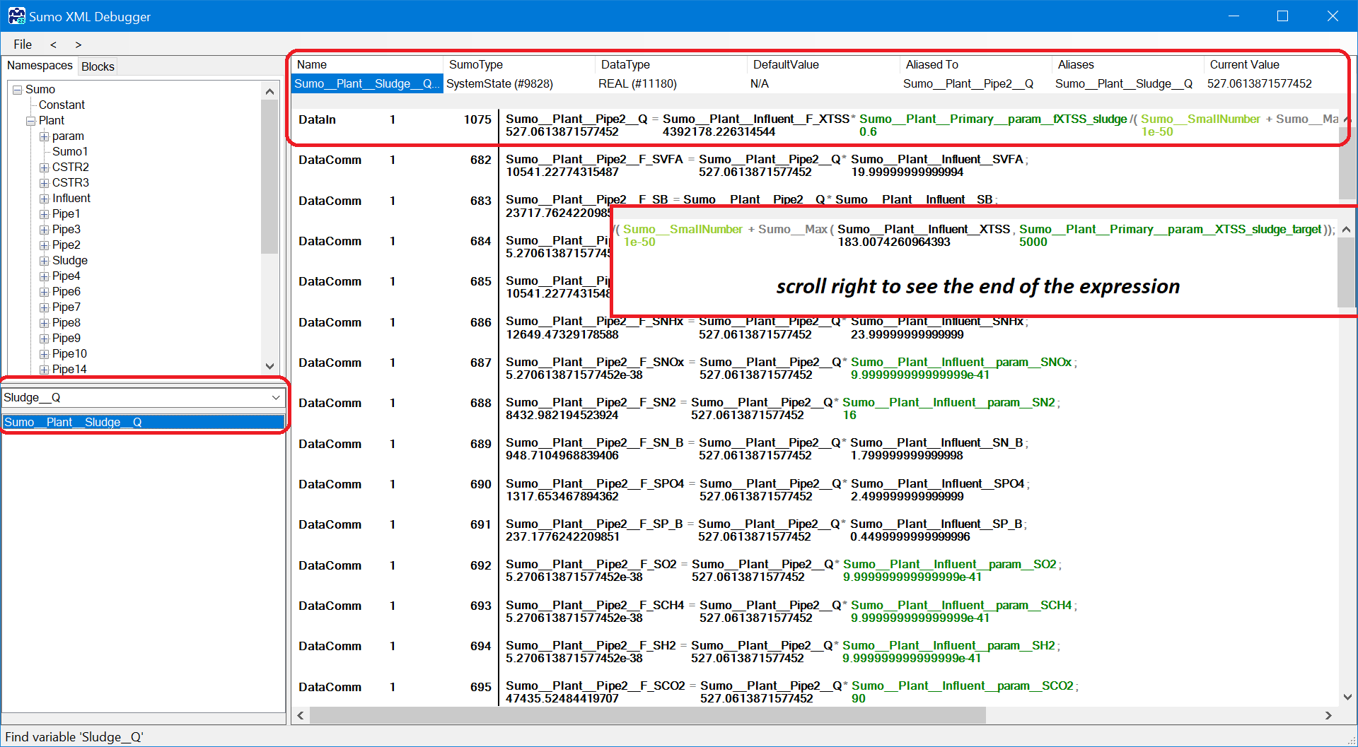
The equation is using full Incode names and below each variable the current value is indicated. This way the variable using wrong values in the calculation can be identified.
The variables used in the expressions are color coded for easier identifying them:
- red: investigated variable
- blue: state variables
- black: systemstates
- green: parameters
- light green: system constants
- grey: functions
Note: there is a glitch if the investigated variable is an alias (has an Aliased To) so the Aliased to variable has to be clicked (in this case it is Pipe2__Q).
¶ Find the name
To find out the name of the variable used in the calculation the Sumo Outputs can be used. On the bottom left panel select the Symbols/Raw and type in the variable name after selecting the (F_XTSS and select Influent):
Remember to set the Advanced|Variable identifier back to Names to see that F_XTSS stands for TSS mass flow.
¶ Where is the issue?
If the first expression (Sludge Q = influent TSS mass flow * removal percent/sludge TSS concentration) is not helping (as the only systemstate is the Influent__F_XTSS) the tool has the feature to follow up on a variable: just click on it and you get the same information for the variable as you can see below for the Influent__F_TSS. On this page the investigated variable is highlighted with red letters. Next to the File menu there are two button for Back and Forward between the already checked variables. Using the Back menu the tool goes back to Sludge__Q variable calculation (XML Figure 9).
Under the calculation of the investigated variable all the equation is listed where the variable is used in the expression (highlighted with red on the right hand side).
This way on a step-by-step basis you can figure out which calculation or which input parameter is wrong.