¶ Gas transfer model
Please cite as: Bencsik D., Wadhawan T., Házi F., Karches T. (2024). Plant-Wide Models for Optimizing the Operation and Maintenance of BTEX-Contaminated Wastewater Treatment and Reuse. Environments 11(5), 88. DOI: 10.3390/environments11050088
The equilibrium between the vapor and liquid phases for gases soluble in water is simulated using Fick’s two-film theory, with gas transfer processes described in our biokinetic models to simulate absorption and desorption. The impact of equilibrium processes on state variables is described within the process model’s Gujer matrix. We note that, within the gas transfer equations, standard conditions regarding gases are interpreted as 101,325 Pa for pressure (pNTP) and 293.15 K for temperature (TNTP,K).
The internal gas phase components are simulated in units of mass per liquid volume. This makes mass and component balancing substantially simpler (compared to using the gas volume as the basis). Equation (1) describes the component balance for gas i.
 |
(1) |
FGi,air,inp denotes the mass flow of gas i from the air supply and is calculated based on the composition of the input gas and the air flow based on the ideal gas law, as shown by Equation (2). The equivalent molar mass MMEQ,i of gaseous components is expressed according to the unit mass of the model state variable, e.g. derived from the theoretical oxygen demand in case of CH4.
 |
(2) |
For gas phase mass balancing, the output gas mass flow FGi,air,outp is calculated by Equation (3), where the concentrations expressed per liquid volume must be converted per volume of gas.
 |
(3) |
The volume of the gas phase in the reactors is estimated based on the gas hold-up fraction εgas. The gas hold-up is an input parameter, for which this paper uses a value of 0.01 m3gas m−3 in case of aerated conditions and 0.001 m3gas m−3 regarding non-aerated conditions (Herrmann-Heber et al., 2019). The gas volumes at field conditions and standard conditions (Vgas and Vgas,NTP, respectively) are calculated by Equations (4) and (5).
 |
(4) |
 |
(5) |
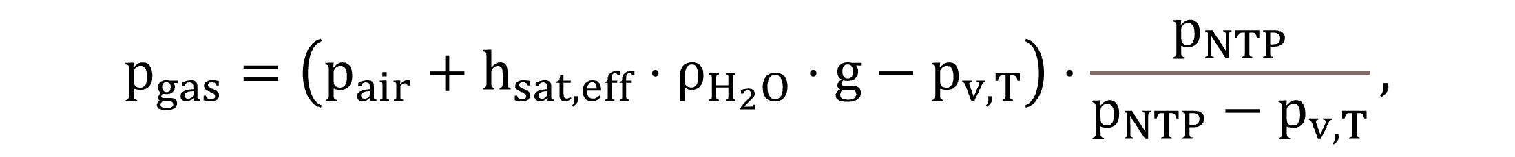
The gas phase pressure pgas is determined by Equation (6) in accordance with EPA guidelines on dissolved oxygen saturation calculations (U.S. Environmental Protection Agency – USEPA, 1989a).
 |
(6) |
The vapor pressure pv,T is calculated by Equation (7) based on the water temperature and Antoine-coefficients, where a multiplication factor is used for unit conversion from mmHg to Pa.
 |
(7) |
The air pressure pair is calculated by the barometric Equation (8), considering the elevation of the facility above sea level hsea (the molar mass of air MMair is converted from the unit g mol−1 to kg mol−1). The parameter Lair for the temperature lapse rate applies a value of 0.0065 K m−1 (Sincero et al., 2002).
 |
(8) |
The calculation of the effective saturation depth depends on whether the tank is aerated, in which case hsat,eff is calculated by Equation (9), and in case there is no aeration, the diffuser submergence hdiff is replaced by the total side water depth (hr). The saturation depth fraction fh,sat,eff may be assigned according to various approaches; the mid-depth concept provides reasonable accuracy in diffused aeration (Stenstrom et al., 2006).
 |
(9) |
For the diffuser depth calculation, the diffuser mounting height is subtracted from the liquid height, according to Equation (10).
 |
(10) |
Unlike liquid phase hydraulic balancing, where the effluent flow is assumed to be equal to the influent, gas phase volumetric balancing needs to take into account the input air flow, as well as the gas transfer activity in the volumetric unit. Equation (11) determines the outgoing gas volumetric flow, Qgas,outp,NTP, which, physically, cannot be negative; this is reflected in the model code (using a maximum function).
 |
(11) |
The volumetric flow of the gas transfer Qgas,transfer,NTP is derived from the summation of the individual gas component transfer molar flows, calculated by Equation (12).
 |
(12) |
Two gas transfer routes are modelled: between the atmosphere and water surface and between the bulk-of-the liquid and bubbles. According to Fick’s first law, the process rate involving the transfer of gas i between the atmosphere and water surface is described by Equation (13), with the driving force of either dissolution or stripping is determined by the difference in the saturation concentration and the liquid phase concentration. The transfer rate of exchange at the gas bubble interface is fundamentally analogous, described by Equation (14).
 |
(13) |
 |
(14) |
Regarding gas transfer through bubbles, the volumetric liquid-side mass transfer coefficients kLai,bub,st,cw—in clean water for a standard 20 °C temperature—and kLai,bub—in wastewater at the field temperature—are calculated by Equations (15) and (16).
 |
(15) |
 |
(16) |
The interfacial transfer area abub is calculated by Equation (17) on a geometrical basis. Based on the literature review, in this study, the bubble Sauter mean diameter dbub is input as 0.003 m for aerated conditions and as 0.01 m under non-aerated conditions (Herrmann-Heber et al., 2019; DelSontro et al., 2015; Jensen et al., 2018).
 |
(17) |
It shall be noted that in cases of fully covered tanks, atmospheric gas transfer is not modelled; the specific surface area abub is extended with the specific contact area between the water surface and the headspace, as shown by Equation (18).
 |
(18) |
On the basis of the Higbie penetration theory, values of the liquid-side mass transfer coefficient kL,i,bub,st,cw are calculated using the respective diffusivities of volatile and soluble gas components by Equation (19) (Roberts et al., 1984), relying on kL,O2,bub,st,cw as a model parameter with the input value of 0.54 m h−1 (Khalil et al., 2021). The parameter for the fraction in the liquid side fkL,i equals 1 for all gases in this study, as they diffuse slowly through the liquid film, with the exception of 0.05 in the case of ammonia, due to its very high solubility (Batstone and Flores-Alsina, 2022).
 |
(19) |
Throughout aerated compartments, the α correction factor is modelled dynamically from process variables representative of wastewater characteristics and loads, explained in the chapter ‘Predictive alpha model’. The θ compensation factor for simulating Arrhenius-type temperature sensitivity in mass transfer is taken as 1.024, following standard procedures in wastewater treatment design (U.S. Environmental Protection Agency – USEPA, 1989a).
For aerated conditions, regarding oxygen, kLaO2,bub is calculated by Equation (20), incorporating a further correction factor for diffuser fouling, an input parameter of aerated unit processes (U.S. Environmental Protection Agency – USEPA, 1989b), which, in practice, is best adjusted knowing the diffuser age and the time of the last cleaning procedure (Jiang et al., 2020). For non-aerated conditions (and regarding coarse bubbles), the correction factor for fouling is not interpreted (equal to one).
 |
(20) |
Regarding oxygen, under aerated conditions, kLaO2,bub,st,cw directly relates to the clean water performance of diffusers; thus, it is derived—according to Equation (21)—from the standard oxygen transfer rate involving air bubbles, SOTRbub.
 |
(21) |
SOTRbub is derived from the specific standard oxygen transfer efficiency SSOTE, which describes the diffused aerator characteristics in clean water, as Equation (22) shows.
 |
(22) |
The prediction of SSOTE is explained in the chapter ‘SSOTE estimation model’.
At the atmospheric interface, calculating the volumetric liquid-side mass transfer coefficients involves the specific mass transfer coefficients (kL) estimated for the liquid surface. The clean water kLai,sur,st,cw at standard conditions and the process water kLai,sur for field conditions are calculated by Equations (23) and (24), respectively.
 |
(23) |
 |
(24) |
The liquid-side mass transfer coefficient regarding the water surface kL,i,sur is determined by Equation (25) using the same principle as for the gas bubble interface, as previously shown by Equation (19).
 |
(25) |
The specific surface area of the liquid asur is calculated by Equation (26), incorporating the multiplication factors fcover for reactor coverage and fwave for turbulence (waviness). The model inputs of 0.54 m h−1 for kL,O2,sur and 1.9 for fwave in this study are adjusted based on the typical measured values of kLaO2,sur found in the relevant literature (Plósz et al., 2003).
 |
(26) |
The water surface area Ar is defined by basin geometry, according to Equation (27).
 |
(27) |
According to Fick’s law, as illustrated previously by Equations (13) and (14), the saturation concentration of a component determines whether the gas–liquid transfer process is driven towards dissolution or stripping. They are calculated by Henry’s law based on the partial pressure of a component, with temperature dependency correction implemented using the van’t Hoff equation (Sander, 2015). The saturation concentrations of gases attributed to the liquid–gas bubble interface Si,bub,sat,st,cw, standardized at 20 °C for clean water (thus requiring temperature conversion from 25 °C, used as the basis of Henry’s law), are modelled based on Equation (28). The variable for process water at field conditions, Si,bub,sat,st, is expressed by Equation (29).
 |
(28) |
 |
(29) |
The β correction factor for impurities in process water uses an input parameter value of 0.95, which is typical of municipal wastewater (U.S. Environmental Protection Agency – USEPA, 1989a).
With regard to the bubble–water interface, partial pressures for standard conditions, ppartial,I,bub,st, and for process conditions, ppartial,i,bub, are calculated by Equations (30) and (31), respectively.
 |
(30) |
 |
(31) |
Equation (32) calculates the molar quantity of gas bubbles per unit liquid volume, ngas,bub.
 |
(32) |
As explained by Equation (33), the pressure at standard conditions, pst,h,sat,eff, is also compensated for the effective saturation depth, as diffuser testing in clean water involves the design submergence (Water Environment Federation – WEF, 2009).
 |
(33) |
The off-gas composition in molar or volume percent units (interchangeable according to Avogadro’s law) may be calculated using Equation (34), expressing Gi,percent, derived from the individual gas component molar concentrations and their sum.
 |
(34) |
The saturation concentrations for the atmosphere–liquid interface, Si,sur,sat,st,cw in the case of clean water and Si,sur,sat regarding process water, are calculated by Equations (45) and (46).
 |
(45) |
 |
(46) |
For the atmospheric saturation concentration calculations, the composition of the atmosphere around the water surface is required. The compositional figures Gi,atm are defined as model constants, measured in volumetric percentages. Equations (47) and (48) quantify the partial pressure of gases in the atmosphere, ppartial,i,sur,st for standardized conditions and ppartial,i,sur for field conditions.
 |
(47) |
 |
(48) |
To sum up, the gas phase composition and the amount of gas dissolving or stripping are dependent on individual gas state variables that impact one another, according to the laws of mass balance. In accordance, the sufficient injection of air or nitrogen gas production will result in other gaseous components (e.g. CO2) stripping out of the liquid.
Nomenclature:
|
α |
alpha (wastewater/clean water) correction factor for mass transfer coefficient |
|
abub |
specific contact area between the gas bubble surface and liquid phase [m2 m−3] |
|
asur |
specific contact area between the surface gas and liquid phase [m2 m−3] |
|
Adiff,sp |
area per diffuser [m2] |
|
Ar |
liquid surface [m2] |
|
β |
beta (wastewater/clean water) correction factor for the saturation concentration |
|
coefflead,h,diff |
leading coefficient in a diffuser submergence correction term [m−1] |
|
coefflin,h,diff |
linear coefficient in a diffuser submergence correction term [m−1] |
|
dbub |
bubble Sauter mean diameter [m] |
|
ddiff |
diffuser density [m2 m−2] |
|
Di,25 |
diffusion coefficient of gas state variable i in water [m2 d−1] |
|
divd,diff |
divisor value in a diffuser density correction term [m2 m−2] |
|
ε |
gas hold-up [m3gas m−3] |
|
expSSOTE |
exponent in SSOTE correlation [d m−3gas] |
|
F |
diffuser fouling factor |
|
fcover |
covered fraction of the reactor surface |
|
FGi |
mass flow of gas phase state variable i [g d−1] |
|
fh,sat,eff |
effective saturation depth fraction |
|
fkL,i |
fraction in the liquid side for the mass transfer of gas state variable i |
|
FLi |
mass flow of liquid phase state variable i [g d−1] |
|
fwave |
waviness factor |
|
Gi |
concentration of gas phase state variable i in off-gas, per liquid volume [g m−3] |
|
Gi,air,inp |
concentration of gas phase state variable i in the air input [%V V−1] |
|
Gi,atm |
concentration of gas phase state variable i in the atmosphere [%V V−1] |
|
Gi,percent |
concentration of gas phase state variable i in off-gas, percentage [%V V−1] |
|
hdiff |
diffuser submergence [m] |
|
hdiff,floor |
diffuser height from floor [m] |
|
Henryi,dt |
temperature dependency factor for Henry coefficient of gas i [K] |
|
Henryi,SATP |
Henry coefficient of gas i, standard (SATP) temperature (25 °C) [mol m−3 Pa−1] |
|
hr |
reactor depth [m] |
|
hsat,eff |
effective saturation depth [m] |
|
hsea |
elevation above sea level [m] |
|
kL,i,bub,st,cw |
liquid-side mass transfer coefficient for gas bubbles, standard conditions [m d−1] |
|
kL,i,sur,st,cw |
liquid-side mass transfer coefficient for liquid surface, standard conditions [m d−1] |
|
kLai,bub |
volumetric mass transfer coefficient for gas bubbles, field conditions [d−1] |
|
kLai,bub,st,cw |
volumetric mass transfer coefficient for gas bubbles, standard conditions [d−1] |
|
kLai,sur |
volumetric mass transfer coefficient for liquid surface, field conditions [d−1] |
|
kLai,sur,st,cw |
volumetric mass transfer coefficient for liquid surface, standard conditions [d−1] |
|
Lair |
temperature lapse rate for air pressure calculation [K m−1] |
|
Li |
concentration of liquid phase state variable i [g m−3] |
|
MMair |
molar mass of air [g mol−1] |
|
MMEQ,i |
equivalent molar mass of gas phase state variable i [g mol−1] |
|
ndiff |
number of diffusers |
|
ngas,bub |
molar quantity of gas bubbles per unit liquid volume [mol m−3] |
|
pair |
air pressure at field elevation [Pa] |
|
pgas |
gas phase pressure [Pa] |
|
pNTP |
pressure at standard (NTP) conditions (101,325 Pa) [Pa] |
|
powd,diff |
power value in a diffuser density correction term |
|
powh,diff |
power value in a diffuser submergence correction term |
|
ppartial,i,bub |
partial pressure of gas state variable i in the gas phase [Pa] |
|
ppartial,i,bub,st |
partial pressure of gas state variable i in the gas phase, standard conditions [Pa] |
|
ppartial,i,sur |
partial pressure of gas state variable i in the atmosphere [Pa] |
|
ppartial,i,sur,st |
partial pressure of gas state variable i in the atmosphere, standard conditions [Pa] |
|
pst,h,sat,eff |
pressure at standard conditions and effective saturation depth [Pa] |
|
pv,T |
saturated vapor pressure of water at temperature T [Pa] |
|
θ |
Arrhenius temperature correction factor for the mass transfer coefficient |
|
Q |
volumetric flow of wastewater [m3 d−1] |
|
Qair,NTP |
air flow at standard (NTP) conditions [m3gas d−1] |
|
Qair,NTP,sp |
air flow per diffuser at standard (NTP) conditions [m3gas d−1] |
|
Qgas,transfer,NTP |
gas transfer flow at standard (NTP) conditions [m3gas d−1] |
|
Qgas,outp,NTP |
off-gas flow at standard (NTP) conditions [m3gas d−1] |
|
rateFi |
mass rate of state variable i [g d−1] |
|
ratei |
reaction rate for the state variable [g m−3 d−1] |
|
rj |
process rate regarding process j (from Gujer matrix) [g m−3 d−1] |
|
Si,bub,sat |
saturation concentration at the gas bubble interface [g m−3] |
|
Si,bub,sat,st,cw |
saturation concentration at the gas bubble interface, standard conditions [g m−3] |
|
Si,sur,sat |
saturation concentration at the atmospheric interface [g m−3] |
|
Si,sur,sat,st,cw |
saturation concentration at the atmospheric interface, standard conditions [g m−3] |
|
SO2 |
dissolved oxygen concentration [gO2 m−3] |
|
SOTRbub |
standard oxygen transfer rate from bubbles [g d−1] |
|
SSOTE |
specific standard oxygen transfer efficiency [% m−1] |
|
SSOTE0 |
intercept in SSOTE correlation [% m−1] |
|
SSOTEasym |
asymptote in SSOTE correlation [% m−1] |
|
T |
liquid temperature [°C] |
|
Tair,K |
field air temperature [K] |
|
TK |
liquid temperature in an SI unit [K] |
|
TNTP,K |
temperature at standard (NTP) conditions (20 °C) [K] |
|
TSATP,K |
temperature at standard (SATP) conditions (25 °C) [K] |
|
Vgas |
gas phase volume [m3gas] |
|
Vgas,NTP |
gas phase volume at standard (NTP) conditions [m3gas] |
|
vj,i |
stoichiometric coefficient of state variable i in process j |
|
Vr |
reactive volume [m3] |
References:
Batstone D., Flores-Alsina X. (2022). Generalised Physicochemical Model (PCM) for Wastewater Processes, IWA Publishing: London, UK. ISBN: 978-1-78040-982-5
DelSontro T., McGinnis D., Wehrli B., Ostrovsky I. (2015). Size Does Matter: Importance of Large Bubbles and Small-Scale Hot Spots for Methane Transport. Environmental Science & Technology 49, pp. 1268–1276. DOI: 10.1021/es5054286
Herrmann-Heber R., Reinecke S. F., Hampel U. (2019). Dynamic Aeration for Improved Oxygen Mass Transfer in the Wastewater Treatment Process. Chemical Engineering Journal 386, 122068. DOI: 10.1016/j.cej.2019.122068
Jensen M. B., Kofoed M. V. W., Fischer K., Voigt N. V, Agneessens, L.M.; Batstone, D.J.; Ottosen, L.D.M. (2018). Venturi-Type Injection System as a Potential H2 Mass Transfer Technology for Full-Scale in Situ Biomethanation. Applied Energy 222, pp. 840–846. DOI: 10.1016/j.apenergy.2018.04.034
Jiang L.-M., Chen L., Zhou Z., Sun D., Li Y., Zhang M., Liu Y., Du S., Chen G., Yao J. (2020). Fouling Characterization and Aeration Performance Recovery of Fine-Pore Diffusers Operated for 10 Years in a Full-Scale Wastewater Treatment Plant. Bioresource Technology 307, 123197. DOI: 10.1016/j.biortech.2020.123197
Khalil A., Rosso D., DeGroot C.T. (2021). Effects of Flow Velocity and Bubble Size Distribution on Oxygen Mass Transfer in Bubble Column Reactors—A Critical Evaluation of the Computational Fluid Dynamics-Population Balance Model. Water Environment Research 93, pp. 2274–2297. DOI: 10.1002/wer.1604
Plósz B. G., Jobbágy A., Grady, C. P. L. (2003). Factors Influencing Deterioration of Denitrification by Oxygen Entering an Anoxic Reactor through the Surface. Water Research 37, pp. 853–863. DOI: 10.1016/S0043-1354(02)00445-1
Roberts P. V., Munz C., Dändliker P. (1984). Modeling Volatile Organic Solute Removal by Surface and Bubble Aeration. Journal of Water Pollution Control Federation 56, pp. 157–163.
Sander R. (2015). Compilation of Henry’s Law Constants (Version 4.0) for Water as Solvent. Atmospheric Chemistry and Physics 15, pp. 4399–4981. DOI: 10.5194/acp-15-4399-2015
Sincero, A. P., Sincero, G. A. (2002). Physical-Chemical Treatment of Water and Wastewater, 1st ed., CRC Press: Boca Raton, FL, USA, 2002. ISBN: 978-1-58716-124-7
Stenstrom M. K., Leu S.-Y., Jiang P. (2006). Theory to Practice: Oxygen Transfer and the New ASCE Standard. In: Proceedings of the Water Environment Federation 2006, 7, pp. 4838–4852.
U.S. Environmental Protection Agency (1989a). Design Manual: Fine Pore Aeration Systems, EPA/625/1-89/023, U.S. Environmental Protection Agency: Cincinnati, OH, USA.
U.S. Environmental Protection Agency (1989b). Summary Report: Fine Pore (Fine Bubble) Aeration Systems, EPA/625/8-85/010; U.S. Environmental Protection Agency: Cincinnati, OH, USA.
Water Environment Federation (2009). Design of Municipal Wastewater Treatment Plants MOP 8, 5th ed., McGraw-Hill Education: Alexandria, VA, USA. ISBN: 978-0-07-166358-8.
¶ SSOTE estimation model
Aeration is one of the most energy-intensive processes at water resource recovery facilities, therefore it is essential to apply a model representative of wide air flow ranges and various aerator configurations, for quantifying the efficiency of diffusers.
The main purpose of modelling aeration efficiency is to be able to properly evaluate oxygen transfer that depends on several physical dimensions within a treatment plant, and varying air flow requirements due to changes in loading – essential for process design involving diurnal influent flow patterns and optimization of treatment plants using dynamic simulation.
Numerous empirical correlations have been developed to describe aerator performance in the field of municipal wastewater treatment, with regression parameters specific to types and manufacturers. Standard oxygen transfer efficiency (SOTE) is a function of the mass transfer coefficient kLa, and research on bubble columns has shown that kLa may be correlated using a power function with superficial gas velocity that is the product of air flow and the reactor area (Shah et al., 1982).
Models have been implemented for calculating SOTE directly in function of air flow and other operational parameters. One approach is applying a polynomial regression equation, relating SOTE to air flow rate per diffuser (air flux), and the depth and density of diffusers (Hur, 1994). This equation has later been modified by the addition of a natural log function to provide a better correlation between SOTE and air flux. (Frank et al., 2009).
Efforts have also been made to apply correlations for the diffuser depth-related aeration efficiency, or specific standard oxygen transfer efficiency (SSOTE) by dimensional analysis (Gillot et al., 2005).
Regarding previously developed correlations, air flux is limited within the ranges used for model calibration and they shall not be extrapolated outside of them. And using logical functions to set strict threshold levels for variables may lead to potential numerical issues when utilized in a dynamic wastewater simulator.
This chapter presents a novel empirical model for estimating SSOTE based on an exponential formula, with the aim of bounding SSOTE between equipment-specific limits; ensuring that it is applicable for virtually any setting of air flux. Correction factors are used to account for diffuser submergence and density.
¶ Methodological Approach
The proposed model was designed to reflect the behavior of fine and coarse bubbles considering previous studies on diffused aeration systems.
Concerning fine bubble aerators, SSOTE is known to drop significantly with increased air flow rate (Morgan et al., 1960). With increasing air flow, size of the air bubbles increases – reducing their specific contact surface and retention time; along with the greater interference of rising bubbles (Ippen et al., 1954; Ellise et al., 1980; Stenstrom et al., 1981).
On the other hand, coarse bubble diffusers show an increasing trend of SSOTE with increasing air flow, as the superficial contact area increases due to bubbles breaking up as a result of higher turbulence (Eckenfelder, 1959).
The general expression selected to model SSOTE in function of air flux is shown below:

Where, SSOTE0: Intercept in SSOTE correlation (%/m)
SSOTEasym: Asymptote in SSOTE correlation (%/m)
expSSOTE: Exponent (absolute value) in SSOTE correlation (-)
Qair,NTP,sp: Normalized air flow per diffuser (m3/d at NTP)
The novelty of this proposed formula is that with any air flux input, the calculated SSOTE will always be capped between the values of the intercept and the asymptote. In case of fine bubbles, the asymptote (value of SSOTE achieved with an infinitely large air flux) is lower than the intercept (SSOTE value with zero air flux). When modelling coarse bubbles, the asymptote is higher than the intercept, as they show the opposite trend of SSOTE in function of air flux. The diffuser-specific air flux Qair,NTP,sp quantifies air flow per number of diffusers:

Where, Qair,NTP: air flow at standard (NTP) conditions (m3/d at NTP)
ndiff: number of diffusers
Further paper research was conducted to integrate the influence of commonly available diffuser characteristics into the model. The absolute transfer efficiency, SOTE increases with diffuser depth, because of the longer contact time of bubbles, and the increased driving force due to the greater partial pressure of oxygen (Mavinic et al., 1974). It is also known that SOTE does not increase linearly with depth, especially in tanks deeper than 8 meters (Pöpel et al., 1994), therefore the proposed SSOTE correlation was extended by a correction term for diffuser submergence:
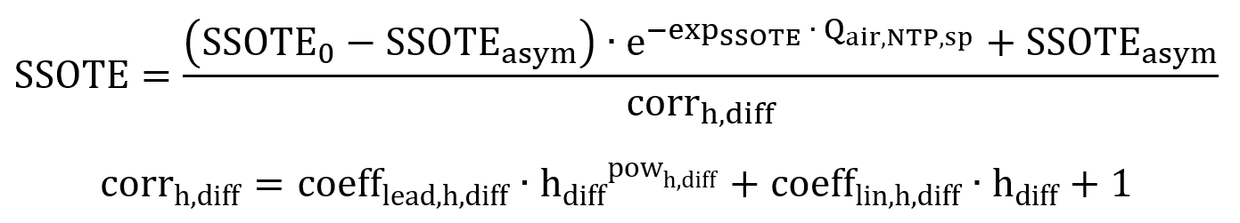
Where, hdiff: Diffuser submergence (m)
coefflead,h,diff: Leading coefficient (1/m)
powh,diff: Power value (-)
coefflin,h,diff: Linear coefficient (1/m)
It has been investigated that in fine bubble aeration, increasing the diffuser floor coverage raises SSOTE (Wagner et al., 1998), as the residence time of bubbles increases with a more evenly distributed mixing profile. A correction term for diffuser density is also applied to the presented correlation, only for modelling fine bubble diffusers:
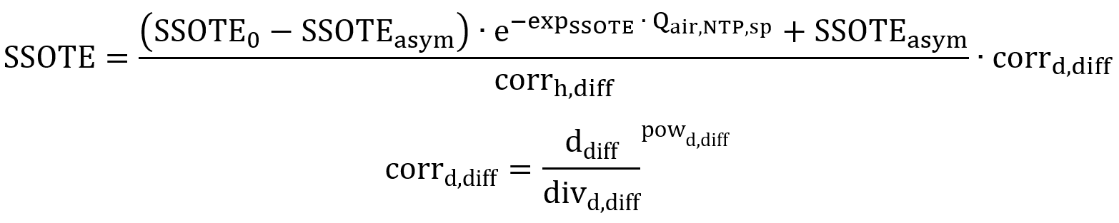
Where, ddiff: Diffuser floor density (m2 diffuser/m2 tank)
divd,diff: Divisor value (m2 tank/m2 diffuser)
powd,diff: Power value (-)
The diffuser floor density ddiff is the ratio of the total diffuser area to the tank surface:

Where, Adiff,sp: area per diffuser (m2)
Ar: liquid surface (m2)
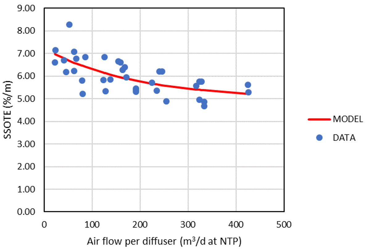
Following model development, a generalized model calibration was carried out based upon data collected from extensive aeration literature review, regarding a type of coarse bubble, and five different types of fine pore diffuser applications (Fig. 1). The Solver add-in from Microsoft Excel was utilized for curve fitting, with the target of minimizing the sum of errors squared, between the measured and correlated SSOTE.
Model validation was performed comparing air flow measurements from two water resource recovery facilities, with the commercial simulation package Sumo 19.3, with dissolved oxygen, diffuser configuration and alpha factor as model inputs.
A Microsoft Excel-based tool was prepared to provide an interface for automated re-estimation of correlation parameters based on diffuser manufacturer specification sheets or plant measurement campaigns, developed using the Visual Basic for Application programming language. For details see Tools in Sumo.
References:
Eckenfelder W. W. (1959). Factors affecting the aeration efficiency of sewage and industrial wastes. Sewage and Industrial Wastes 31(1), pp. 60–70.
Ellise S., Stanbury, R. (1980). The Scale-up of Aerators. In: Symposium on The Profitable Aeration of Waste Waters, 3, BHRA Fluid Engineering Report, Cranfield, Bedford, England.
Frank K., Davies G., Shirodkar N., Sauvageau A. (2009). Aerating a high rate low SRT activated sludge reactor: coarse or fine bubble aeration – how about a hybrid? In: Proceedings of the Water Environment Federation 2009, 8, pp. 7215–7224. DOI: 10.2175/193864709793957382
Gillot S., Capela-Marsal S., Roustan M., Héduit A. (2005): Predicting oxygen transfer of fine bubble diffused aeration systems – model issued from dimensional analysis. Water Research 39(7), 1379–1387. DOI: 10.1016/j.watres.2005.01.008
Hur D. S. (1994). A computer program for optimal aeration system design for activated sludge treatment plants. M.S. Thesis, University of California, Los Angeles.
Ippen A. T., Carver C. E., Dobbins W. E. (1954). Basic factors of oxygen transfer in aeration systems. Sewage and Industrial Wastes 26(7), pp. 813–829.
Mavinic D. S., Bewtra J. K. (1974). Bubble size and contact time in diffused aeration systems. Journal of Water Pollution Control Federation 46, pp. 2129–2137.
Morgan P. F., Bewtra J.K. (1960). Air diffuser efficiencies, Journal of Water Pollution Control Federation 32, pp. 1047–1059.
Pöpel H. J., Wagner M. (1994). Modelling of Oxygen Transfer in Deep Diffused-Aeration Tanks and Comparison with Full-Scale Plant Data. Water Science and Technology, 30(4), pp. 71-80. DOI: 10.2166/wst.1994.0161
Shah Y. T., Kelkar B. G., Godbole S. P., Deckwer W. D. (1982). Design Parameters Estimation for Bubble Column Reactor, AIChE Journal, 28(3).
Stenstrom M. K, Gilbert, R. G., (1981). Effects of Alpha, Beta and Theta Factor upon the Design, Specification and Operation of Aeration Systems. Water Research 15, pp. 643-654.
Wagner M., Pöpel H. J. (1998). Oxygen transfer and aeration efficiency – influence of diffuser submergence, diffuser density, and blower type. Water Science and Technology 38(3), DOI: 10.1016/S0273-1223(98)00445-4
¶ Predictive alpha model
Please cite as: Bencsik D., Takács I., Rosso D. (2022). Dynamic alpha factors: Prediction in time and evolution along reactors, Water Research 216, 118339. DOI: 10.1016/j.watres.2022.118339
The performance of aeration – one of the costliest processes at water resource recovery facilities – is heavily impacted by actual wastewater characteristics and diffuser usage, that are commonly taken into account using the α and F factors, respectively. The α factor changes depending on loading – meaning both in time and spatially (e.g., along plug flow reactors). In standard design practice it is often considered as a fixed number, or at best, a predefined time series. There is a need to more accurately predict α for the design and operation of WRRFs. The objective of this study is to propose such a method by the use of process modelling, adjusting to diurnal and seasonal variations in hydraulic and organic loading.
¶ Methodological Approach
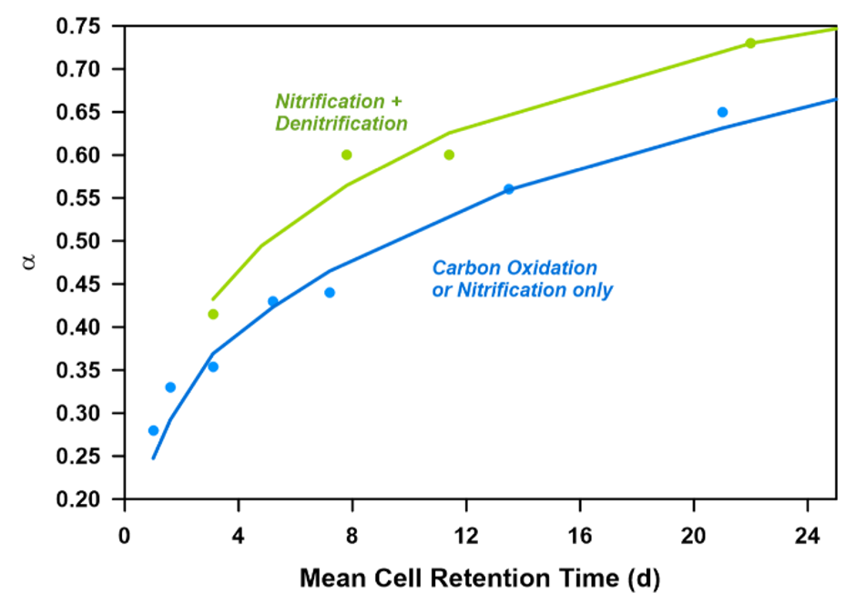
The concept of dynamic prediction of the α factor is based on a “typical” or “average” degradable component. As this component sorbs to flocs and degrades kinetically in the system, α increases towards the clean water value. This novel concept was selected because change of the α value in space and time cannot be directly linked to any of the state variables (readily biodegradable substrate, ammonia etc.) that models typically deal with. The model developed by the authors takes into account the dependence of α on sludge retention time in the form of degradation kinetics, the effect of organic loading (influent filtered COD), the presence or absence of anoxic zones and the effect of high MLSS found in certain, e.g., MBR technologies.
Data was collected from results of off-gas measurement campaigns, clean water and process water tests; while also relying on aeration literature review (Rosso et al., 2008; Leu et al., 2009; Baquero‐Rodríguez et al., 2018). Reconciliation of data was carried out according to IWA Good Modelling Practice Guidelines (Rieger et al., 2013). The model was then first fitted to averaged α factor measurements from facilities applying newly commissioned fine pore diffusers – with and without non-aerated selectors – in function of the given plant MCRT values (Figure 1). Suspended solids-related correction in the model was fine-tuned based upon α factor batch tests without loading. The modelled behaviour of α in terms of influent filtered COD was adjusted based on diurnal continuous off-gas testing.
A variant of the BSM1 test configuration (Alex et al., 2008) was set up in Sumo21© and used to evaluate potential CAPEX and OPEX (energy and effluent fines) savings due to using the proposed predictive α model (and the resulting more correct blower sizes and control) instead of fixed overly cautious or too optimistic design values.
Mini_Sumo was selected as a biokinetic model – in favor of an up-to-date gas transfer concept, extended by Sumo’s blower and pump models to assess energy and associated costs. Throughout model simulation, α factor for aged diffusers (αF, including fouling factor) was used for results interpretation – assigning a fixed value of 0.75 for F.
¶ Results and Discussion
In the authors’ first study the model was run to dry weather steady-state using Sumo’s combined global and local solvers, followed by 5 weeks of repeated dry weather diurnal weeks (GT Figure 3). Three runs were performed in order to obtain the required blower sizes for the following different design methods:
- Kinetic-based model prediction (space and time varying αF):
average calculated αF at 0.48, 0.5 and 0.53 in AER1, AER2 and AER3 - Cautious design:
αF set to 0.3, 0.4 and 0.5 in AER1, AER2 and AER3 - Optimistic design:
αF set to 0.5, 0.6 and 0.7 in AER1, AER2 and AER3
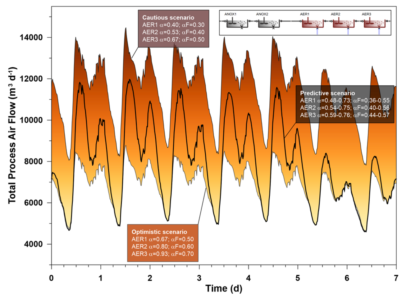
Compared to the cautious design example that estimates an accumulated blower energy consumption of 45,846 kWh, the time and location-specific αF prediction use case determines only 34,765 kWh, suggesting 24% savings on operational costs. Although the weekend air demand estimated by the optimistic design approach shows good agreement with the predictive method, it only assumes 31,362 kWh of required blower energy; and it would potentially lead to insufficient air supply during most of the week.
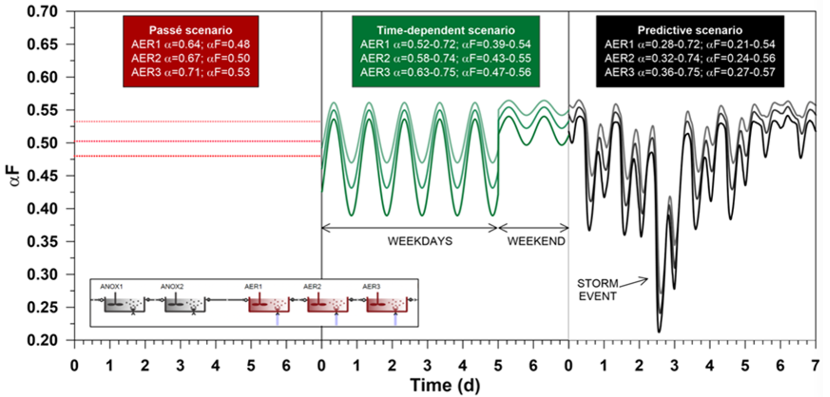
In another experimental study, model-predicted αF was compared to best sinusoidal approximation. A sinusoidal approximation for αF in each reactor was created using a cos() function. The sinusoidal αF variation was based on the dynamically predicted model results, by matching the average and the timing and value of the highest αF peak in each reactor separately for weekdays and weekend days.
After steady-state and 5 weeks of dry weather loading, a 6th week was simulated where the flow (and therefore the load) on Wednesday was doubled. The sinusoidal αF prediction was not changed during the overload period. The blower used was the best design (12,000 m3/h). The air flow requirement for this run can be compared to the response of the dynamic prediction run for the same week (GT Figure 4).
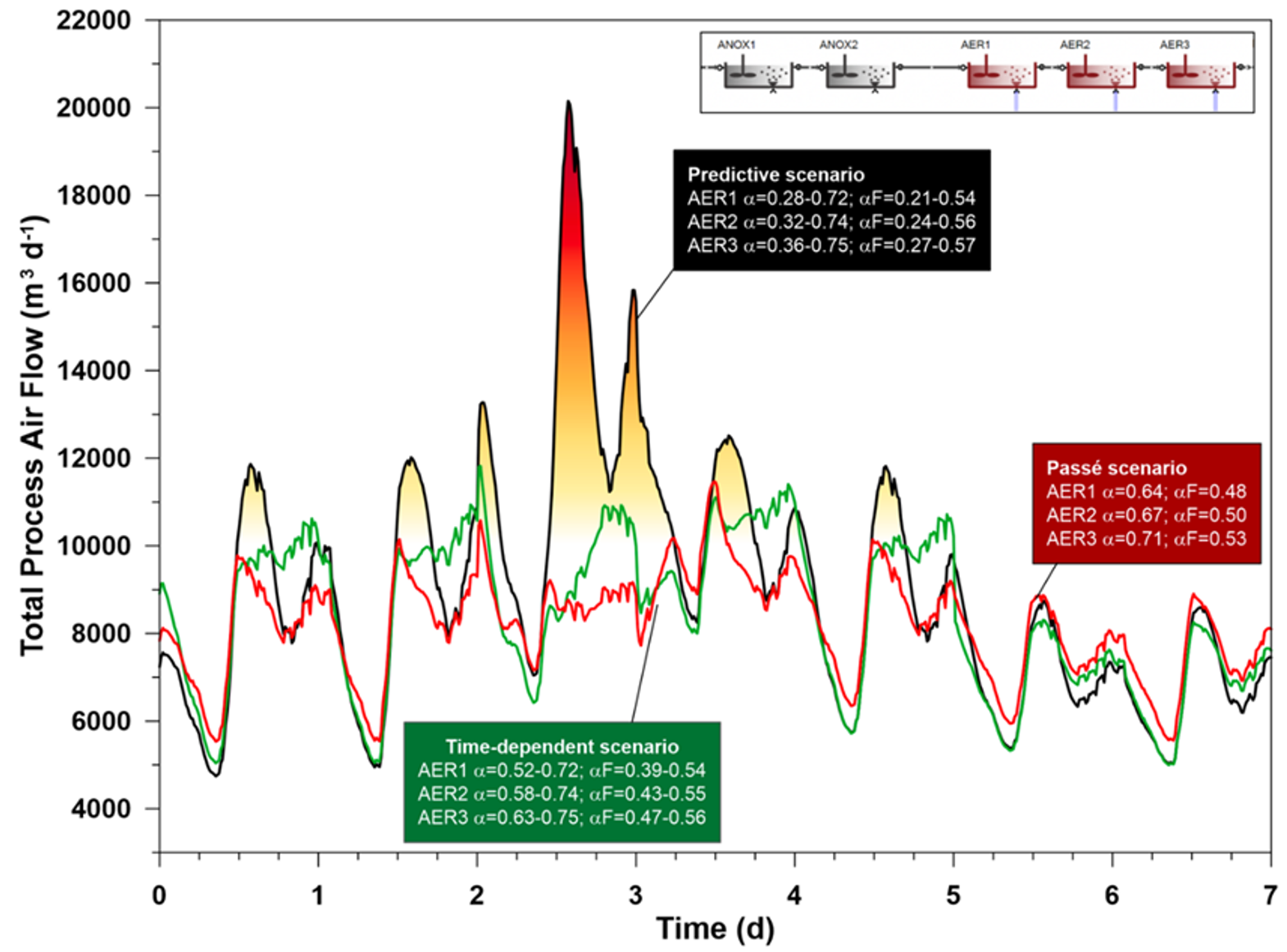
If the load increase is considered, it turns out that 12,000 m3/h blower capacity would in fact not be enough, while the sinusoidal αF design suggests it will suffice. Blower size was not restricted in this run. The predictive approach evaluates (properly) lower αF, and consequently, higher air flow associated with it. The sinusoidal and constant scenarios calculate slightly reduced air flow – they do not account for αF reduction by the sudden load variation (Figure 4), and due to the high hydraulic load ammonia is washed out to a peak of 27 mg N/L in all three scenarios. DO setpoints are maintained in all three scenarios, but in reality, only the dynamic αF case would be able to maintain them, the other two αF presumptions are flawed and consequently the air flow is wrong.
References:
Alex J., Benedetti L., Copp J., Gernaey K., Jeppsson U., Nopens I., Pons M.-N., Rieger L., Rosén C., Steyer J.P., Vanrolleghem P.A., Winkler S. (2008). Benchmark Simulation Model no. 1 (BSM1). In: Report by the IWA Task Group on Benchmarking of Control Strategies for WWTPs, pp. 19–20.
Baquero-Rodríguez G.A., Lara-Borrero J.A., Nolasco D., Rosso D. (2018). A Critical Review of the Factors Affecting Modeling Oxygen Transfer by Fine-Pore Diffusers in Activated Sludge. Water Environment Research 90(5). DOI: 10.2175/106143017x15131012152988
Bencsik D., Takács I., Budai P., Rosso D. (2021). The last barrier to accurate aeration design: The alpha factor – How to predict in time and along the reactor, In: WRRmod2021 conference proceedings, International Water Association (IWA), pp. 130-134.
Leu S.-Y., Rosso D., Larson L.E., Stenstrom M.K. (2009). Real-time aeration efficiency monitoring in the activated sludge process and methods to reduce energy consumption and operating costs. Water Environment Research 81(12), pp. 2471-81. DOI: 10.2175/106143009X425906
Rieger L., Gillot S., Langergraber G., Ohtsuki T., Shaw A., Takács I., Winkler S. (2013). Guidelines for using activated sludge models. IWA, Scientific and Technical Report No. 22.
¶ SumoBioFilm model
The SumoBioFilm model is used in the following process units:
- BAF
- MBBR
- MABR
- Trickling filter
- Granular SBR
¶ Model implementation
The biofilm model of Sumo (called SumoBioFilm) is developed by Dynamita to provide a reasonable simplified description of biofilm systems for wastewater process modelling. The first modelled technology was the Moving bed bioreactor solution, called MBBR.
The simplifications are the following:
- Fixed biofilm thickness with n layers:
The model uses an average biofilm thickness, thus layer thickness via the layer number as input parameter. Inside the biofilm layers the biofilm is ideally mixed, similar to the CSTR (Continuously Stirred Tank Reactor). - 1D model
The model has 1D extension with the homogeneous biofilm layers. In the basic reactor unit biofilm composition is uniform. - Active media surface model
Input parameters are required to provide information about the active surface of the media used in the technology. The specific surface, the media fill ration and the media water displacement parameters define the biofilm amount with the biofilm thickness. - Biofilm specific mass
The biofilm specific mass describes the TSS content of the biofilm growing on the active surface of the media as g TSS/m2 active media surface. This parameter defines the biofilm dry matter content which is kept during the simulation with a built in TSS controller. - Detailed mass transfer description for the biofilm
The model uses 4 different transport mechanism to describe the mass transfer inside the biofilm: - Diffusion of components and convection for enthalpy:
- between bulk and biofilm,
- between biofilm layers
- Active solids transfer between biofilm layers
- Attachment from the bulk phase to biofilm
- Detachment from the biofilm to the bulk phase
¶ Biofilm characterization
The biofilm can be characterized via the following parameters at the input setup:
| Biofilm and biofilm carrier parameters | |||
| Symbol | Name | Default | Unit |
| n | Number of biofilm layers | 3 | - |
| zF | Biofilm thickness | 300 | micron |
| zBL | Boundary layer thickness | 30 | micron |
| XTSS,spec | Biofilm specific mass | 10 | g TSS.m-2 biofilm |
| Asp.carrier | Specific surface of biofilm carrier | 500 | m2 biofilm.m-3 loose media |
| icarrier | Ratio of reactor volume filled by carriers | 0.5000 | m3 loose media.m-3 reactor |
| Vsp.carrier | Water displaced by carrier | 0.1800 | m3 loose media.m-3 reactor |
From the advanced view the biofilm density can be set:
| Biofilm density | |||
| Symbol | Name | Default | Unit |
| ρF | Biofilm density | 1020 | kg.m-3 |
The active media/carrier surface (considered as biofilm surface) and volume is calculated as follows:
| Biofilm carrier parameters | |||
| Symbol | Name | Default | Unit |
| Acarrier | Total biofilm carrier surface* | icarrier*Asp.carrier*L.V** | m2 media/biofilm surface |
| Vcarrier | Volume displaced by the carrier | icarrier*Vsp.carrier*L.V | m3 |
| * Equals to biofilm surface. ** L.V is the reactor total volume - including liquid phase, media/carrier volume and biofilm volume. Input parameter, technically it is the depth x tank surface. |
|||
Biofilm volume is calculated based on the above calculated biofilm surface:
| Biofilm properties | |||
| Symbol | Name | Expression | Unit |
| AF | Total biofilm surface | Acarrier | m2 biofilm |
| zL | Biofilm layer thickness | zF/n | m |
| Biofilm volume | |||
| Symbol | Name | Expression | Unit |
| VF | Biofilm volume | AF*zL* | m3 biofilm |
| * With additional sum for each biofilm layer (can be expressed as: n * AF * zL) | |||
The biofilm dry matter (TSS) content is defined as follows:
| Biofilm properties | |||
| Symbol | Name | Expression | Unit |
| XTSS,target | Target TSS concentration in biofilm | XTSS,spec * AF/VF * (ρF * cg,kg)/ρH2O | g TSS.m-3 biofilm |
| XTSS,F | Dry matter content of biofilm | M,XTSS,film,total/(VF*ρF) | g.kg-1 |
| * cg,kg is the unit conversion between kg and g ** ρH2O is the density of water *** M,XTSS,film,total is the total TSS mass stored in the the biofilm (ideally as XTSS,target * VF) |
|||
¶ Example based on default parameters
Based on the default parameters in 1 m3 reactor volume there is 250 m2 active carrier surface with 300-micron biofilm thickness providing a total 0.075 m3 biofilm. The total TSS in the biofilm is 2500 g TSS, thus the XTSS,target is 33333 g/m3 biofilm, which is 3.26 g/kg dry matter content (based on the 1020 kg/m3 biofilm density).
¶ Mass transfer
The mass transfer processes are differentiated between the different components based on the specification of the component in the models. The components can be soluble, colloidal or particulate based on their characteristic. The following processes are considered in the SumoBioFilm model for each component type for the 2 main transfer surfaces:
| Processes | On the surface between bulk and biofilm | Inside biofilm (surface between biofilm layers) | ||||
| Soluble components | Colloidal components | Particulate components | Soluble components | Colloidal components | Particulate components | |
| Diffusion |
X |
X |
|
X |
X |
|
| Solids transfer |
|
|
X |
|
|
X |
| Attachment of solids |
|
|
X |
|
|
|
| Detachment of solids |
|
|
X |
|
|
|
| TSS controller |
|
|
|
|
|
X |
In general, the mass transfer processes specified above are described based on the driving force as concentration difference on the two sides of the transfer surface multiplied by a specific transfer coefficient.
¶ Separation models
¶ Volumeless separation model
Mass balance based algebraic models with various input parameter combinations.
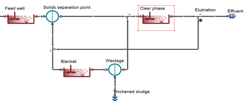
¶ Three compartment separation model
The models are valid for Sumo1, Sumo2, Sumo2C and Sumo2S models.
This is a complex unit composed with a feed well, a point separator, a clear water compartment and a sludge blanket (SM Figure 1). These three compartments are CSTR with diffused aeration and input DO units. Feedwell and Sludge blanket are reactive for model reactions. In the feed well, polymer can be added.
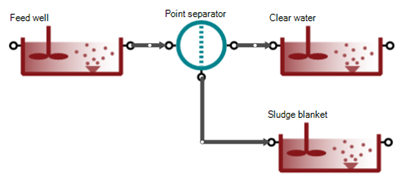
In sludge flow or sludge concentration specified models an elutriation flow allow natural or forced circulation of flow from sludge blanket to clear liquid to account for the diffusion of soluble components.
¶ Input parameters
Settings parameters are:
- Total volume
- Feed well volume
- Sludge blanket volume
- Sludge solids concentration or Sludge flow
- Effluent solids concentration or Percent solids solids removal (with and without polymer)
Polymer addition parameters are:
- Polymer concentration
- Rate of precipitation with polymer
- Half-saturation of polymers in flocculation
- Half-saturation of colloidal substrate in flocculation with polymers
- Half-saturation of polymers for solid percent removal improvement
Other parameters are:
- Surface of clarifier
- Elutriation rate:
- 0: no elutriation;
- Few % - natural elutriation
- 1: forced elutriation to wash out VFA
¶ Polymer addition concepts
The polymer addition in this process unit impacts the solid removal in two ways:
¶ The colloidal substrate flocculation
The flocculation of colloidal substrates with polymer processes rates are calculated in the code sheet.
rateFLOC,CB,polymer = qFLOC,polymer * MsatFLOC,polymer * MsatCB,KFLOC,polymer * Xpolymer
rateFLOC,CU,polymer = qFLOC,polymer * MsatFLOC,polymer * MsatCU,KFLOC,polymer * Xpolymer
The rates are first order to polymer concentration and have a Monod saturation function on the colloidal substrate and on the polymer concentration.
The half saturation of polymers in flocculation is the half of the optimal dose to reach the maximum flocculation rate.
¶ The removal efficiency of solids
The removal efficiency will be adjusted between the Solids percent removal without polymer and Solids percent removal with polymer values given by the user
The adjustment between the two values uses a Monod function with the half-saturation of polymers for solid percent removal improvement parameter
¶ Triple exponential settling model
¶ Parameter estimation
The 1-D layered settling models used in various separator process units in Sumo employ parameters that are based on Vesilind zone settling velocity lab tests. Following the release of Sumo21, continued effort was made to facilitate the use of this approach. Users are more familiar with the sludge volume index (SVI) which is also a routine lab test. Despite its shortcomings form the modeling aspect, it is a widely available data, as opposed to zone settling velocity tests.
On one hand, empirical correlation functions from literature had been evaluated and three of them (Ozinsky and Ekama, 1995; Härtel and Pöpel, 1992 – DOI:10.2166/wst.1992.0128; Daigger, 1995 – DOI:10.2175/106143095X131231) were chosen to be included as an option to estimate Vesilind settling parameters from SVI values, if the user opts to do so, instead of entering Vesilind parameters directly.
On the other hand, an Excel tool has been developed to ease the processing of the Vesilind lab test data. The key part of this task is to identify the linear section of the individual settling curves and fit a line to this part in order to derive the settling velocity for the specific MLSS concentration (the lab test is executed for a range of MLSS). The tool is capable of automatically performing this fit, after the user enters/imports the test data. The applied algorithm uses first and second differentials (akin to first and second derivatives of continuous functions) in various resolutions and a ranking mechanism based on the goodness of the fits and the range of the data used for the fits. Manual refining is also an available option. Once this task is done for all the available settling tests, the tool collects the corresponding MLSS and settling velocity data pairs and makes a fit to come up with the maximum Vesilind settling velocity and the hindered settling parameter.
¶ Dewaterability model
A mechanistic modelling approach is identified and developed to simulate and predict sludge bound water content and dewaterability in the context of whole plant simulation. Currently, whole plant simulators do not predict bound water content and use a simplified solid-phase separation unit to model mechanical dewatering. The model unit requires cake solids concentration and solids capture percentage as inputs. This limits the use of the model to only one operational scenario unless these inputs were changed accordingly to reflect the impact of operation or new technologies in dewatering performance. The composition of wastewater and the biological, chemical and physical transformational forces applied to it play a role in how bound water content of the sludge and its dewaterability changes. We successfully applied a model to predict the bound water content and dewaterability in terms of cake solids at a large wastewater treatment plant, Virginia Initiative Plant operated by Hampton Roads Sanitary District, Virginia, USA.