¶ Introduction
Add-on packages are dedicated process units to cover different technologies or areas such as mobile carrier technologies or detailed sewer network modeling. The chapter provides description about these models.
The addons are available for download on our website.
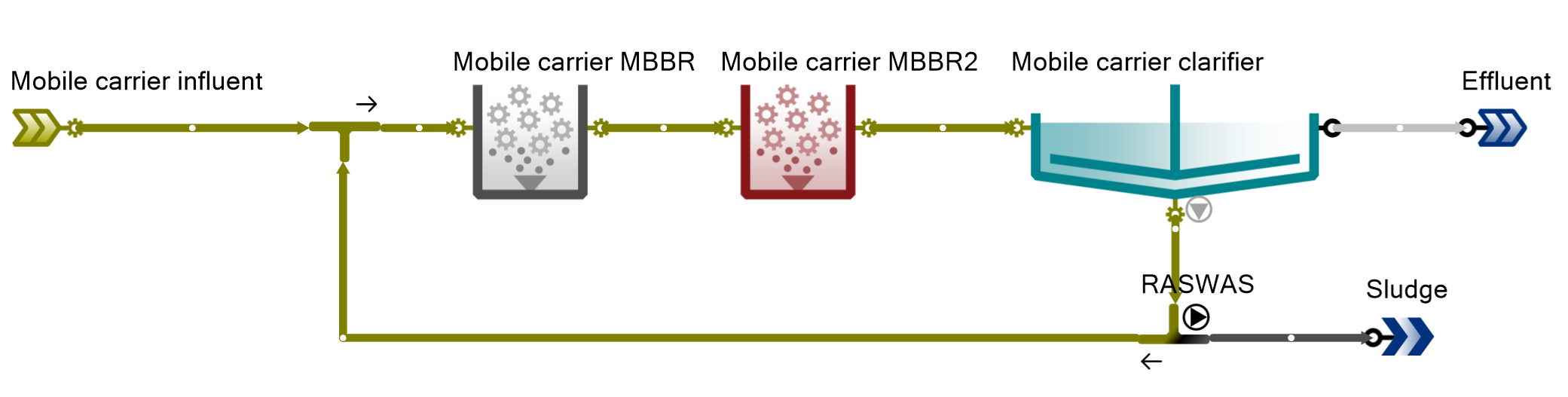
¶ Mobile carrier model
Mobile carrier can be described as free moving, submerged biofilm carrier which can leave the reactor boundaries with the biofilm attached to it.
Mobile carrier (MC) model is the extension of the SumoBioFilm© model by allowing the carrier and the attached biofilm to move between process units. The model uses Xcarrier variable to calculate the amount of carrier and attached biofilm transported via connections. The sub-model allows the simulation of recirculation, back mixing, media removal and addition.
Biofilm carrier migration model describes reactor performance, Water Science & Technology, 75.12, 2017, Joshua P. Boltz, Bruce R. Johnson, Imre Takács, Glen T. Daigger, Eberhard Morgenroth, Doris Brockmann, Róbert Kovács, Jason M. Calhoun, Jean-Marc Choubert and Nicolas Derlon
¶ Sewer model
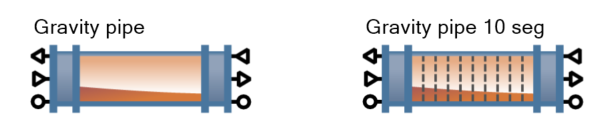
The sewer network add-on contains a gravity pipe and a pressure pipe process unit, a service cover and compatible gas flow elements. The pipes are consider as a single reactor or as a plug flow reactor of 10 segments with fixed biofilm or sediments on the wetted surface area.
In gravity sewers, the gas phase is allowed to flow both directions – same as sewage and counter direction as well. The service cover predicts fresh air intrusion and gas transfer.
¶ Gravity pipes
The gravity pipe segment is implemented as a 3-3 input and output ports process unit: one input for sewage, one for gas (same direction as sewage), one for gas (counter direction). Same 3 for outputs.
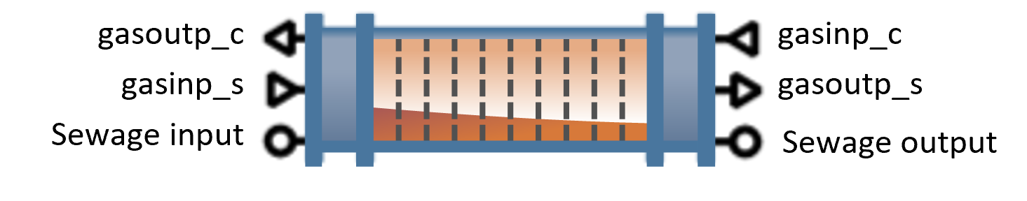
A gravity pipe with 10 segments can be used to reproduce the plug flow behaviour. Sewage flows in one direction, no recirculation is possible. Influent always enters the first segment. The ports with circles are for the liquid phase, the ports with triangles are for the gas phase. The triangles themselves show the direction of gas flow at that port.

The length, pipe diameters and fraction of liquid in segments can be modified in parameter inputs.
¶ Headspace and air movements
Gravity sewer pipes are not filled 100% liquid, headspace is accounted. Mass transfer between the sewage and gas phase takes place with a fixed kLa (13 d-1 for gas bubbles and 7.6 d-1 at liquid surface).
Gas phase is allowed to flow both directions – same as sewage and counter direction as well. This should be implemented in a way that changing flow direction should be possible during simulation, no retranslation should appear.
Based on the influent gas flows from both directions, the process unit calculates the ultimate gas flow. In this implementation, only Q (m3/d) gas is considered. The resultant Qair depend on two cases:
- If one of the gas input flows is higher, it backflow the smaller flow. The air flow in the pipe segment is then the higher input flow. The same side pipe segment output flow is equal to the sum of the two input flows. The counter side output flow is null.
- If the two input flows are equal, the two output gas flows are then equal to the input gas flows, and Qair in the sewer segment is null. The mass flows are not mixed.
¶ Biofilm
A fixed biomass is modeled as a one-layer biofilm with a fixed thickness. The biofilm cover the wetted surface area.

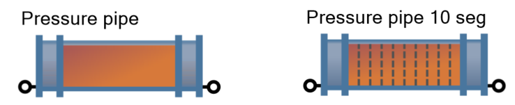
¶ Pressure pipes
Pressure pipes are similar to gravity pipes but does not have any headspace and are filles to 100%.
Pressure pipes with a single reactor or with 10 segments can be selected. A fixed biofilm or sediments on the wetted surface area is considered. Mass transfer between the sewage and bubbles gas phase takes place with a fixed kLa (13 d-1), so that a stripping can occur in a downflow process.
¶ Gas combiner

The air flows are summed, and the mass flow is calculated adequately.
¶ Gas divider


The air flow is divided with a fix flow (pump) or proportionally to the input flow and the mass flow is calculated adequately.
¶ Sewer side flow combiner
Similarly to the pipe segment, the side flow combiner is implemented as a 3-3-3 input and output ports process unit. The liquid flows entrance from the left and the top of the process unit. The liquid flow (input through the circles ports) is represented by the grey lines and its direction is indicated by the arrow below the graphic.
The ports with triangles are for the gas phase and the triangles themselves show the direction of gas flow at that port.

The liquid flow output is the sum of the two liquid flows inputs.

The air flow output depends on two cases:
- If one of the input is smaller than the two others, the flow outputs to the corresponding port. The resultant Qair is the sum of the three gas influent flows (calculated at each integrated step). This flow goes to the smallest gas input side, the two other side flow outputs being then zero. An applied example of this case is represented below.

- In case of the two smallest flows are equal, the resultant Qair in these two directions is the half of the maximum flow plus the input port flow. An applied example of this case is represented below.

¶ Service cover
The service cover mimics an air input (gasventinp) or output (gasventoutp) from or to the outside of the sewer network. The air flows from or to outside the sewer network (gasventoutp and gasventinp) are fixed as parameters. The rest of the service cover is a 3-3 input and output ports process unit as pipe segment, but with no volume and non-reactive.


The air flow outputs to the smallest gas input side and to the gasventoutp (if not null). Two cases may happen:

- The two air flows from the sewer network are equal (gasinp_s..Q = gasinp_c..Q)
- If the net gas ventilation input is positive (gasventinp - gasventoutp), the air flow in both sides is then the gas input flow of the counter direction plus the half of the net ventilation input flow ((gasventinp..Q - gasventoutp..Q)/2).

- if the output net ventilation flow is positive, the effective gas ventilation output is the minimum of the user entry and the total sewer gas input flows. The output air flow in the same side and counter sewer flow direction is then the gas input flow of the counter direction deduced by the half of the net ventilation output flow.

- One of the air flow from the sewer network is higher than the other (gasinp_s..Q ≠ gasinp_c..Q).
- If the net gas ventilation input is positive, the sum of the three input flows is backflowing through the smallest sewer input flow direction.

- if the output net ventilation flow is positive, the effective gas ventilation output is the minimum of the user entry and the total sewer gas input flows. The output air flow in the smallest sewer input flow direction is the total of the sewer gas input flows deducted by the net ventilation output flow.

¶ Densified Sludge Model
This add-on includes a Densified sludge separator process unit to simulate the granules selection obtained with a hydrocyclone. A specific model extension is required to simulate separate biological reactions in the flocs and granules: Sumo2 with the granule extension model.
¶ Model description
The concept is based on the aerobic granular sludge modeling approach described by Baeten et al. (2018) wherein separate modelling state variable components are assigned for floccular and granular organism groups. The diffusion resistance of substrate into the granules is accounted for using higher “apparent” half-saturation coefficients for granular components. The selective retention and accumulation of granules is predicted by the model as a result of the differential effect on the floccular and granular organism groups of biological selector zones and external selectors, for example wasting from the overflow of hydrocyclones.
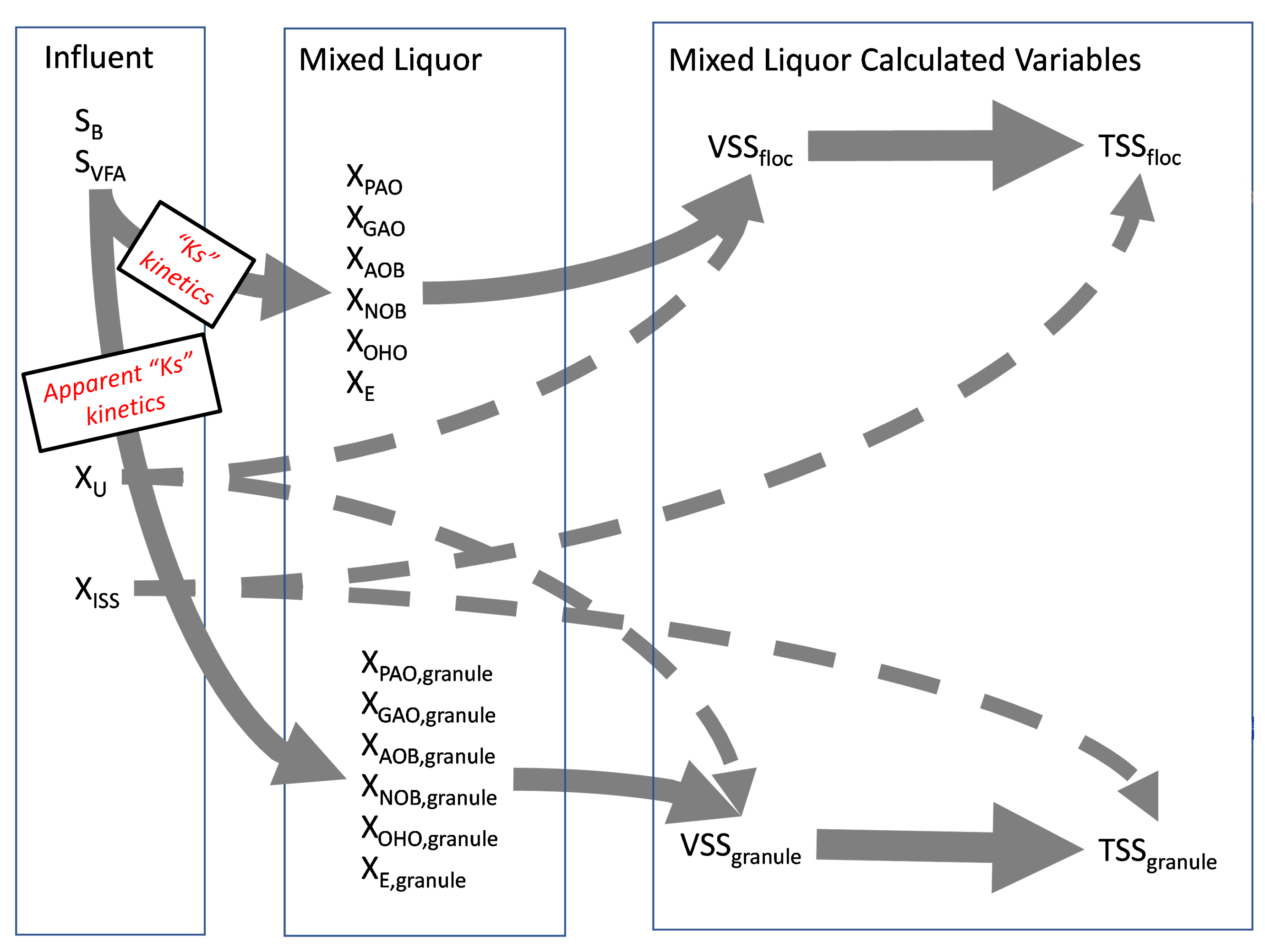
The granule fraction is calculated as a function of the relative ratio of granular to total organism groups (granules + flocs) and by assigning portions of influent particulate material to either the floccular or granular groups.
Under normal circumstances, the floccular components of ordinary heterotrophs (XOHO), and PAO and GAO carbon storing organisms (XCASTO) will dominate the growth processes because the model applies a “Diffusion Resistance” parameter to the growth of granular organisms. This diffusion resistance accounts for the reduced access to substrate and oxygen in the inner layers of the granules. It is applied using the “apparent Ks” concept described by Baeten et al. (2018). For example, in the equation below the Monod saturation term for some substrate “S” is defined with the half-saturation coefficient “MsatS” increased proportionally to the diffusion resistance “DR”. The default value of DR is 3 which implies a 300% increase in the half-saturation coefficient.

In fact the term (Ks*DR) acts as the “apparent Ks” investigated by Baeten et al. Table 1 shows how this might be applied in a simplified model matrix. Figure 1 provides a conceptual framework for how modeling direction of influent substrate to growth of floccular and granular organisms in the mixed liquor can then be used to calculate the densified fraction of the mixed liquor.
Table 1 - Gujer matrix presenting separate state components for floccular and granular PAOs, storage products (PHA) as well as “apparent Ks” applied to VFA sequestration and O2 utilization in granules
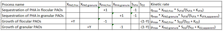
Because the higher “apparent Ks” has less impact when substrate concentrations are high, the model will simulate the beneficial effects of an internal selector for sludge densification. It is then easy to model the benefits of an external selector to enhancing densification, such as a hydrocyclone, in which granular state variables are selectively retained.
¶ Biokinetic model specifics
A granular fraction of the following components has been implemented as state variable:
Table 2 - List of Sumo2_granule specific state variables
| XB,granule | Slowly biodegradable substrate in granule |
| XB,e,granule | Slowly biodegradable substrate from biomass decay - granule |
| XU,granule | Particulate unbiodegradable organics in granule |
| XPHA,PAO,granule | Polyhydroxyalkanoates (PHA) stored by PAOs in granule |
| XPHA,GAO,granule | Polyhydroxyalkanoates (PHA) stored by GAOs in granule |
| XE,granule | Endogenous decay products in granule |
| XE,ana,granule | Anaerobic endogenous decay products in granule |
| XOHO,granule | Ordinary heterotrophic organisms (OHO) in granule |
| XCASTO,granule | Carbon storing organisms (CASTO) in granule |
| XMEOLO,granule | Anoxic methanol utilizers (MEOLO) in granule |
| XAOB,granule | Aerobic ammonia oxidizers (AOB) in granule |
| XNOB,granule | Nitrite oxidizers (NOB) in granule |
| XN,B,granule | Particulate biodegradable organic N (from XB) in granule |
| XN,Be,granule | Particulate biodegradable organic N (from XBe) in granule |
| XN,U,granule | Particulate unbiodegradable organic N in granule |
| XPP,granule | Stored polyphosphate (PP) in granule |
| XP,B,granule | Particulate biodegradable organic P (from XB) in granule |
| XP,Be,granule | Particulate biodegradable organic P (from XBe) in granule |
| XP,U,granule | Particulate unbiodegradable organic P in granule |
| XINORG,granule | Inorganics in influent and biomass in granule |
The biological processes of Ordinary heterotrophic organisms (OHO), Carbon storing organisms (CASTO), Anoxic methanol utilizers (MEOLO), Aerobic ammonia oxidizers (AOB) and Nitrite oxidizers (NOB) have been duplicated from the flocs. The stoichiometric and kinetic parameters for these biological processes are identical in granules and flocs, except for the half-saturation parameters that are multiplied by a diffusion resistance factor. The default values of the diffusion resistance parameters vary between 1, for autotrophic biomasses which are located on the surface of the granule, and up to 4 for ordinary heterotrophic biomass. The variation of these values is representative of the results from Baeten et al. (2018), but the defaults values have been chosen lower than the one calibrated in Baeten et al. (2018). Indeed, their experimental results focused on AGS with an average diameter of 0.55mm, while densified sludge produces granules are mainly smaller, between 0.2 and 0.5mm (Roche et al, 2021).
Note that the model results are very sensitive to these parameters, as demonstrated in the chapter “Calibrating Diffusion Resistance (DR)” of the Quick Tutorial hereafter.
To handle the decay-regeneration of biomass inside the granule, specific biokinetic processes have been implemented:
- Granule OHO growth on decay products in granule (XB,e,granule) with O2, NO2 or NO3 as electron acceptors.
- XB,e fermentation under high and low VFA concentration and by OHOs and PAOs
Furthermore, to give the possibility to user to simulate attachment or detachment on granules processes, a biokinetic process for the “granules to floc net conversion” is added. By default, its kinetic rate “Granule to floc conversion rate” (qgranule,floc) is set to zero. This rate can be set at a positive (detachment) or negative (attachment) value.
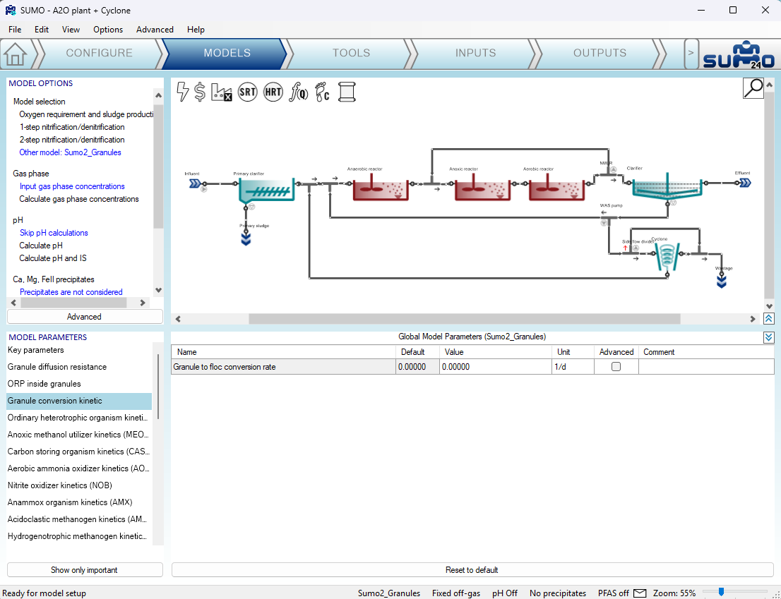
¶ Cyclone model specifics
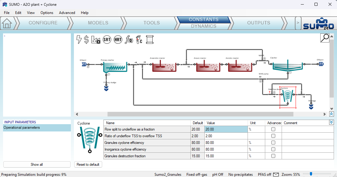
The cyclone model for densified sludge selector must be chosen in the options of the cyclone.
This is a volumeless point separator process unit, that will only mass balance the state variable depending on few parameters:
- Flow split to underflow as a fraction: the default value is 20%, meaning that the underflow of the cyclone will be 20% of the influent flow rate and the overflow will be 80% of the influent flow rate.
- Ratio of underflow TSS to overflow TSS: the default value is 2, meaning that the TSS concentration at underflow is twice the concentration of TSS at the overflow.
- Granule fraction efficiency: the default value is 80%, meaning that 80% of the granules leaving the cyclone are captured at underflow, and 20% are lost at the overflow. (Note: considering the granule destruction fraction of 15% described hereinafter, the mass flow rate of granules at the underflow is calculated as 85% x 80% of the influent mass flow rate of granules.)
- Inorganics cyclone efficiency: the default value is 80%, meaning that inorganics that have a granule size will be selected by 80% to the underflow, in same proportion than granules.
- Granules destruction fraction: the default value is 15%, meaning that 15% of the influent mass flow rate of granules is destroyed by the action of the hydrocyclone, and are missing in the experimental mass balance around the hydrocyclone.
J. Baeten, M.C.M. van Loosdrecht, E. Volcke (2018) “Modelling aerobic granular sludge reactors through apparent half-saturation coefficients.” 146. 134-145. Water Research.
Roche, C., Donnaz, S., Murthy, S., Wett, B., 2021. Biological process architecture in continuous‐flow activated sludge by gravimetry: Controlling densified biomass form and function in a hybrid granule–floc process at Dijon WRRF, France - Roche - 2022 - Water Environment Research - Wiley Online Library. Water Env. Res 2021;e1664.
¶ Quick tutorial: How to use Sumo Densified Sludge Model
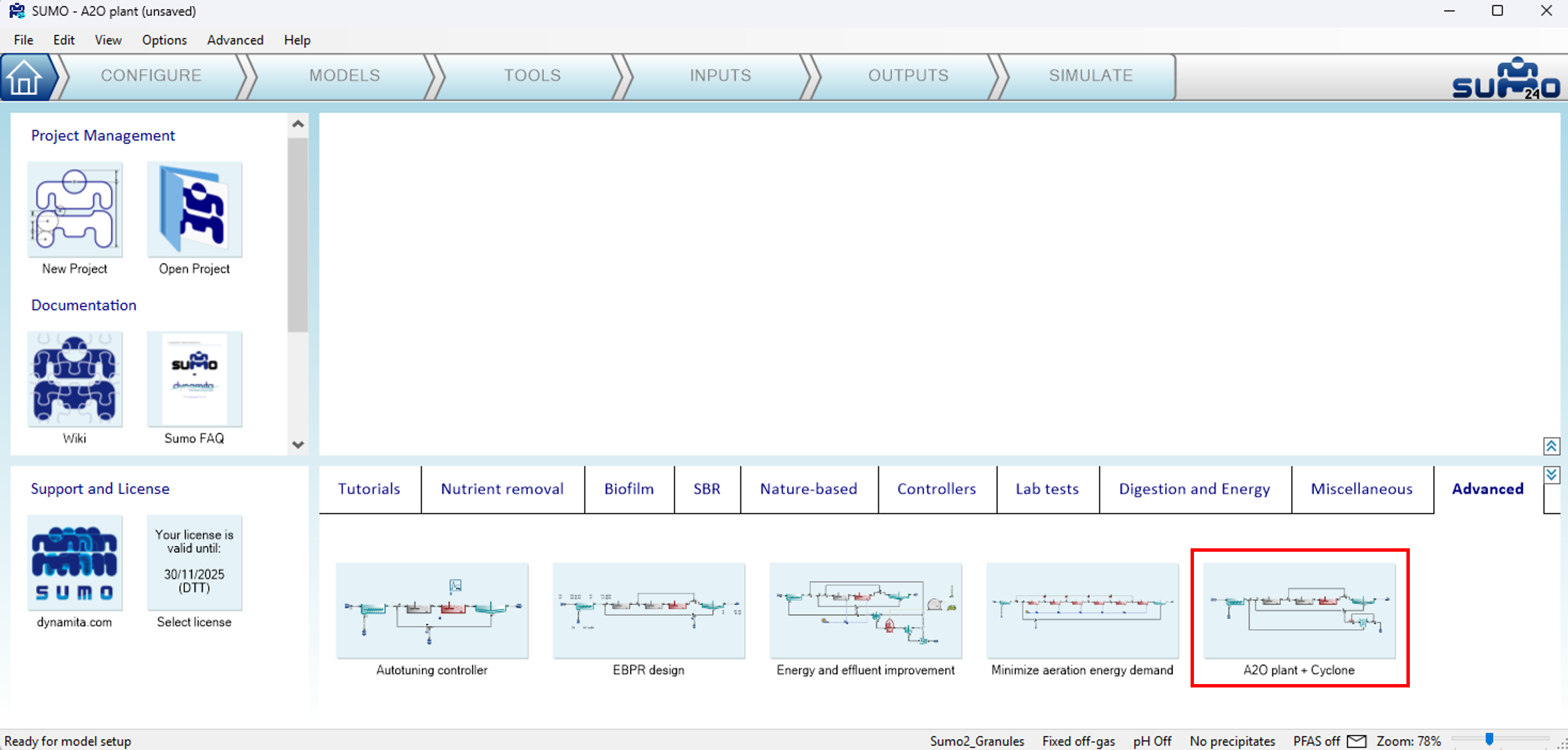
An example with a cyclone configuration can be found under “Advanced” examples. Although, the following tutorial explains step by step how to build such configuration.
¶ Opening an existing example in Sumo
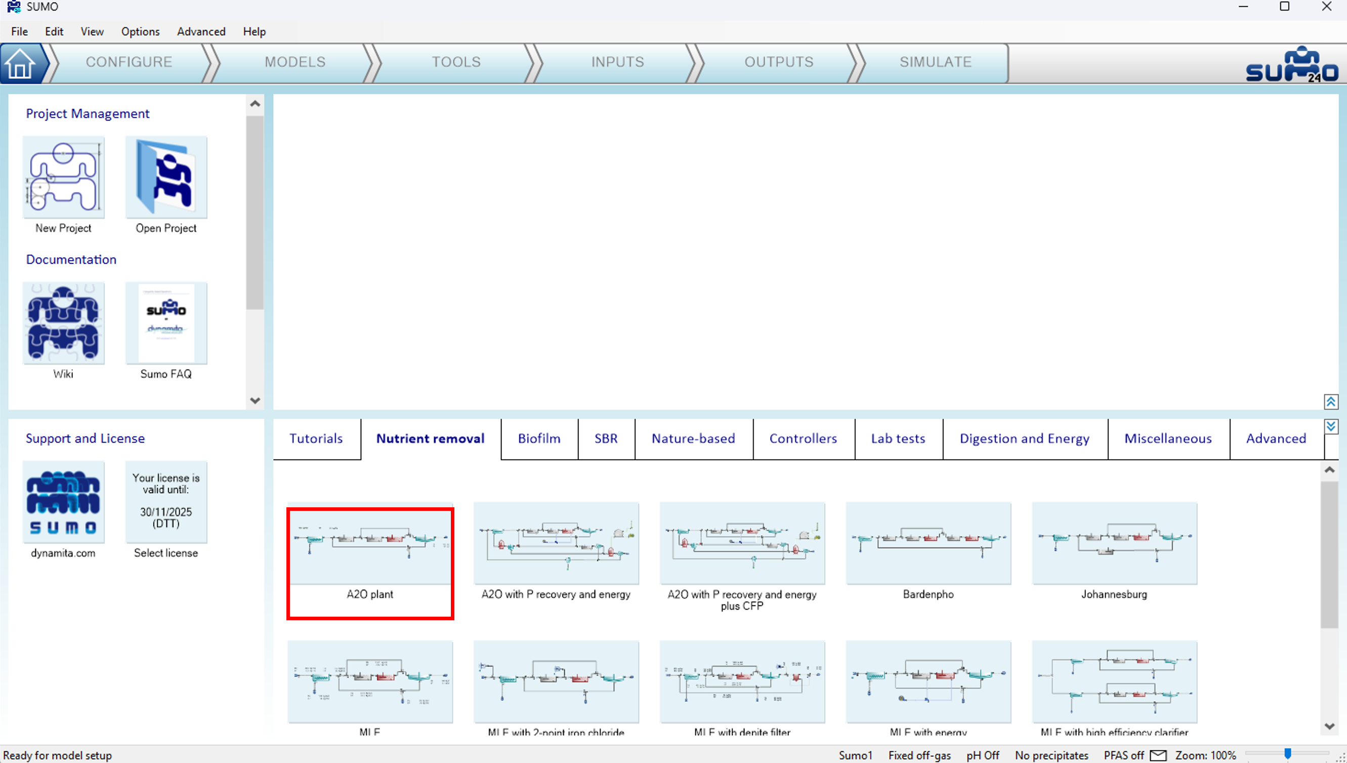
You can modify an existing Sumo model to work with the densification model. In this example, we will select the A2O plant from the list of Examples in the home screen.
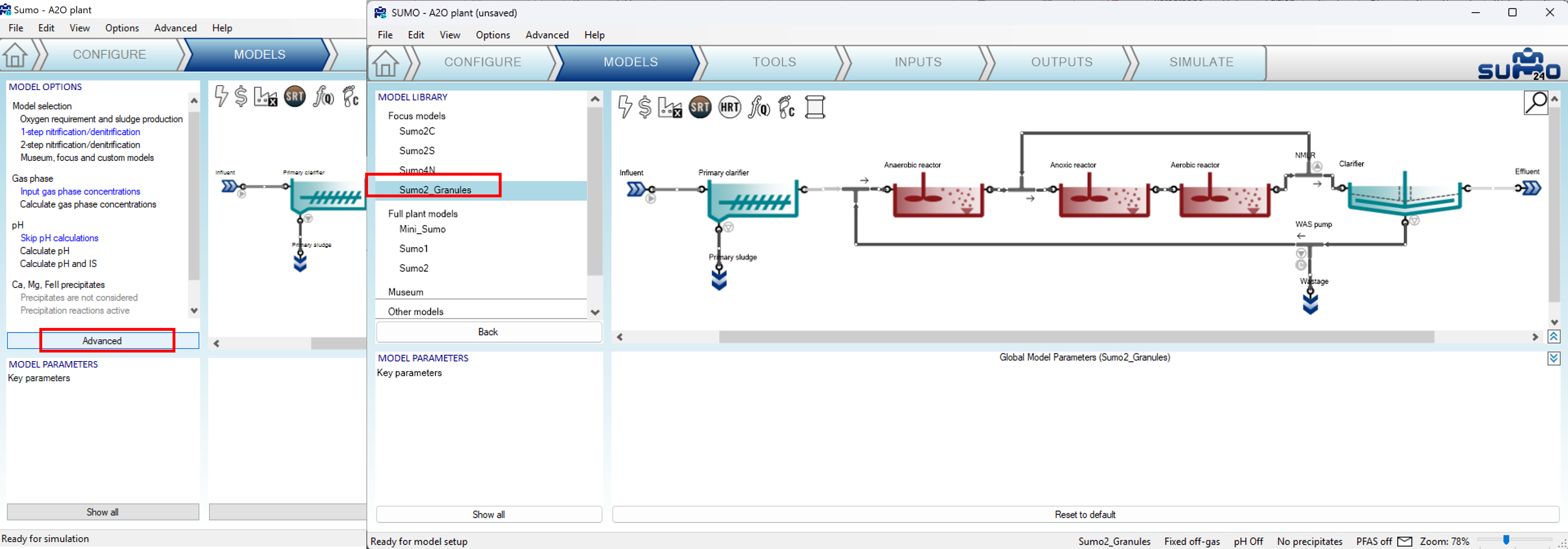
¶ Selecting the Sumo2_Granules biokinetic model
To select the densification biokinetic model, go to the MODELS tab in the Sumo ribbon, select the “Advanced” option, and then the Sumo2_Granules option from the Focus models. This model is based on Sumo2, a 2-step nitrification model, with the modification that certain particulate state variables are divided between floccular and granular components.
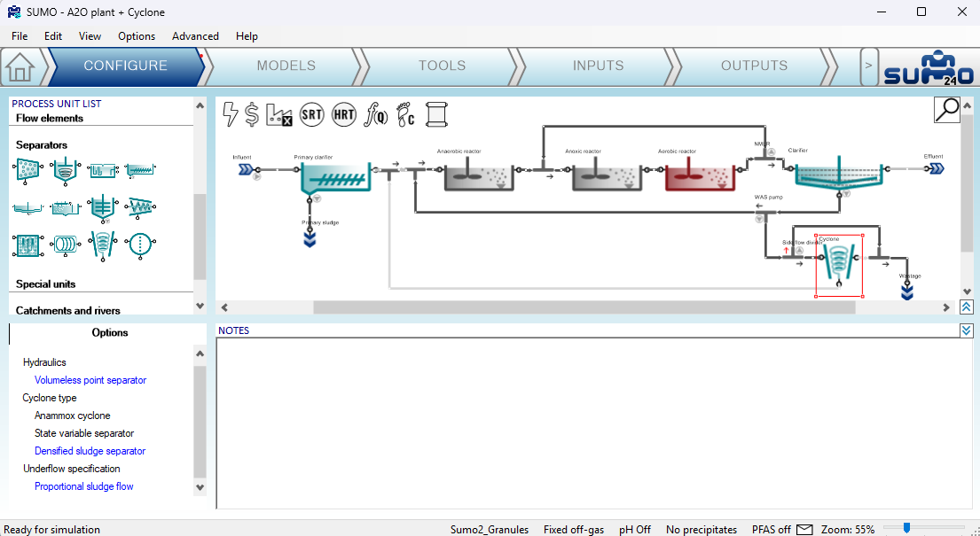
¶ Adding a Cyclone from the Separators elements
To add a hydrocyclone to the flowsheet, select it from the “Separators” in the CONFIGURE tab of the Sumo ribbon. Make sure to select “Densified sludge separator” from the Options in the bottom left pane.
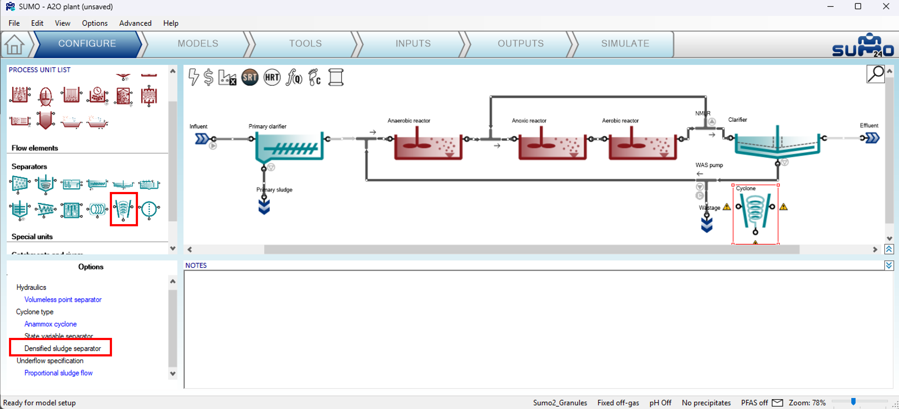
The hydrocyclone is added to the WAS stream together with a “Proportional side flow divider” to enable easy switching “On” and “Off” of the cyclone operations.
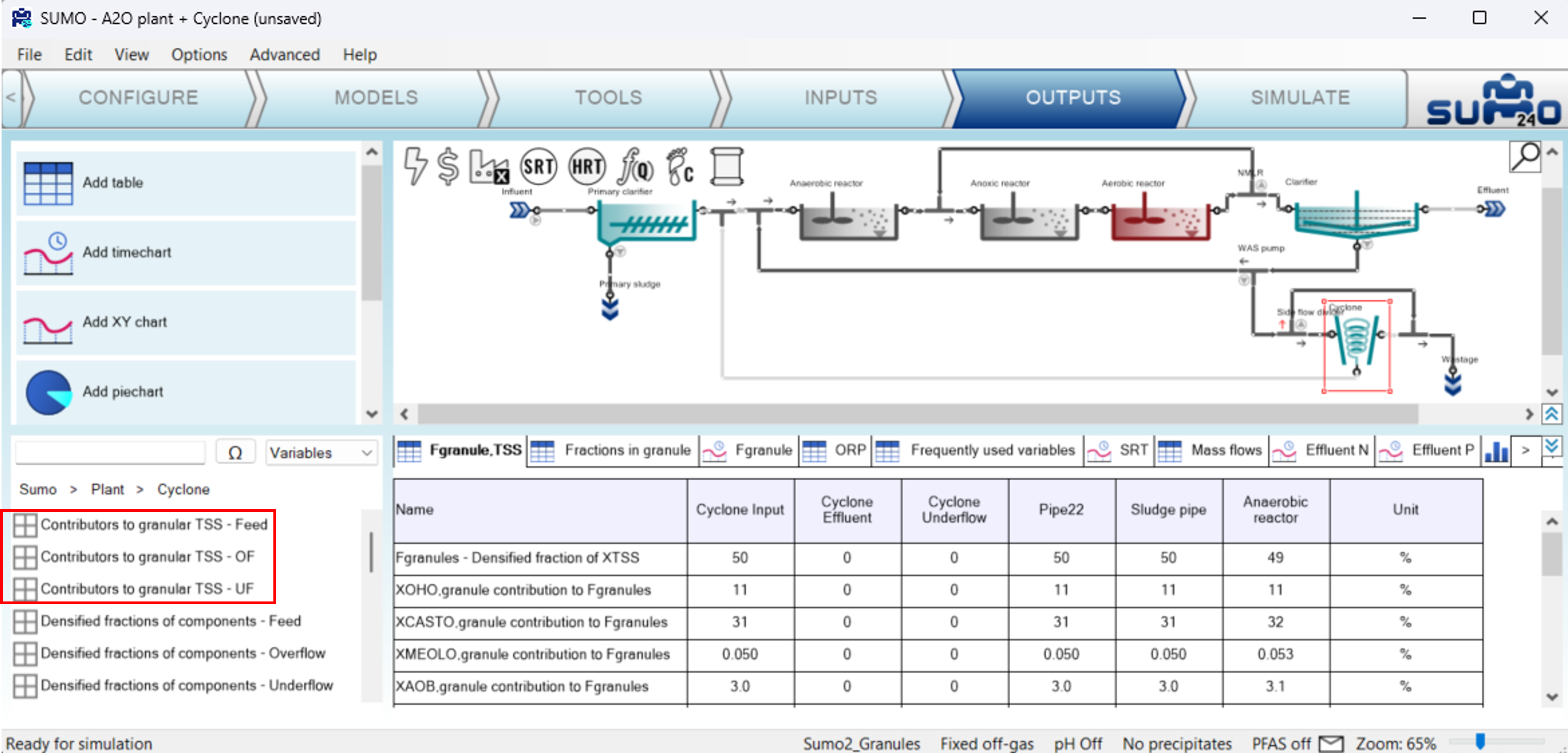
¶ Displaying the Densified Fraction of TSS
In the OUTPUTS tab, select the Cyclone element. Create a table and drag and drop the “Contributors to granular TSS” into the table for each of the Feed, Overflow and Underflow. You can drag and drop the input and output ports of the cyclone to create the different columns.
¶ Create scenarios for Cyclone “On” and “Off” scenarios
In the INPUTS tab of the Sumo ribbon, select the proportional side flow divider immediately upstream of the cyclone and check the “Scenario” box.
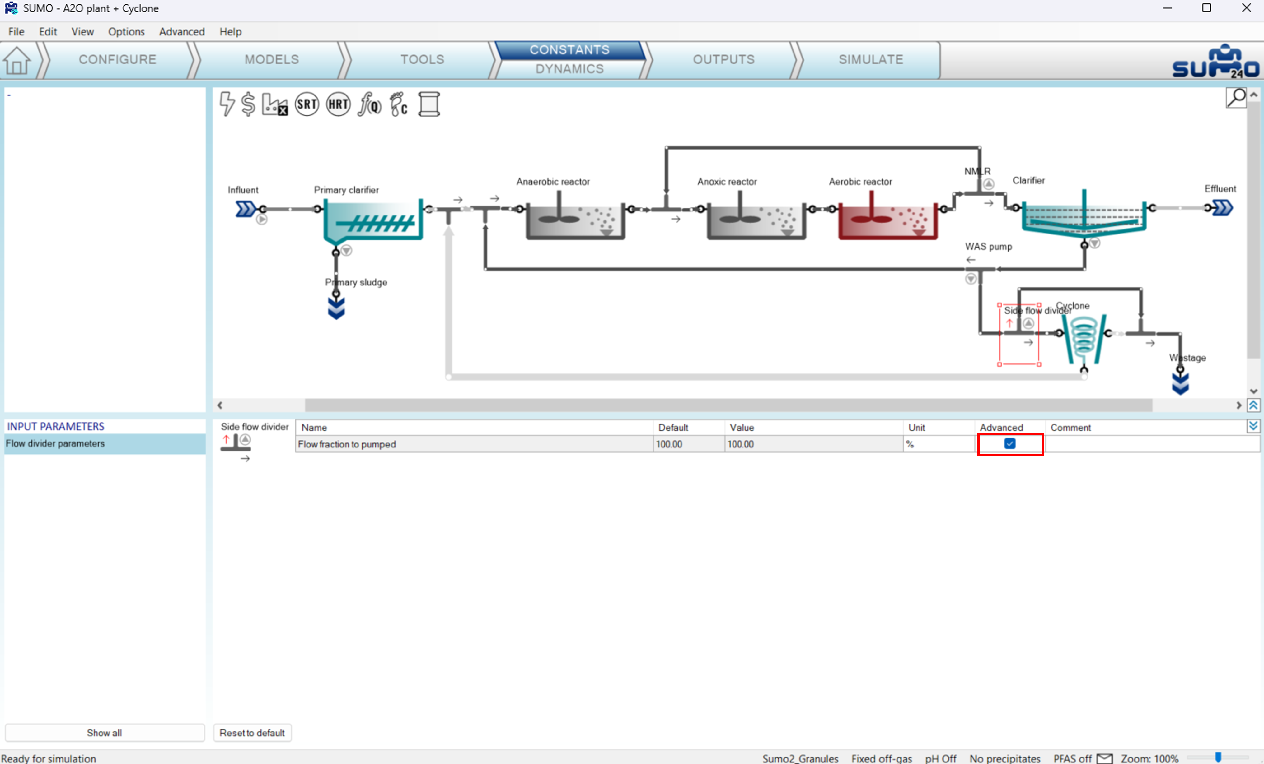
In the SIMULATE tab, this parameter will now appear as an option in the bottom left pane. Create and name two scenarios to represent Cyclone “On” and “Off” operations.
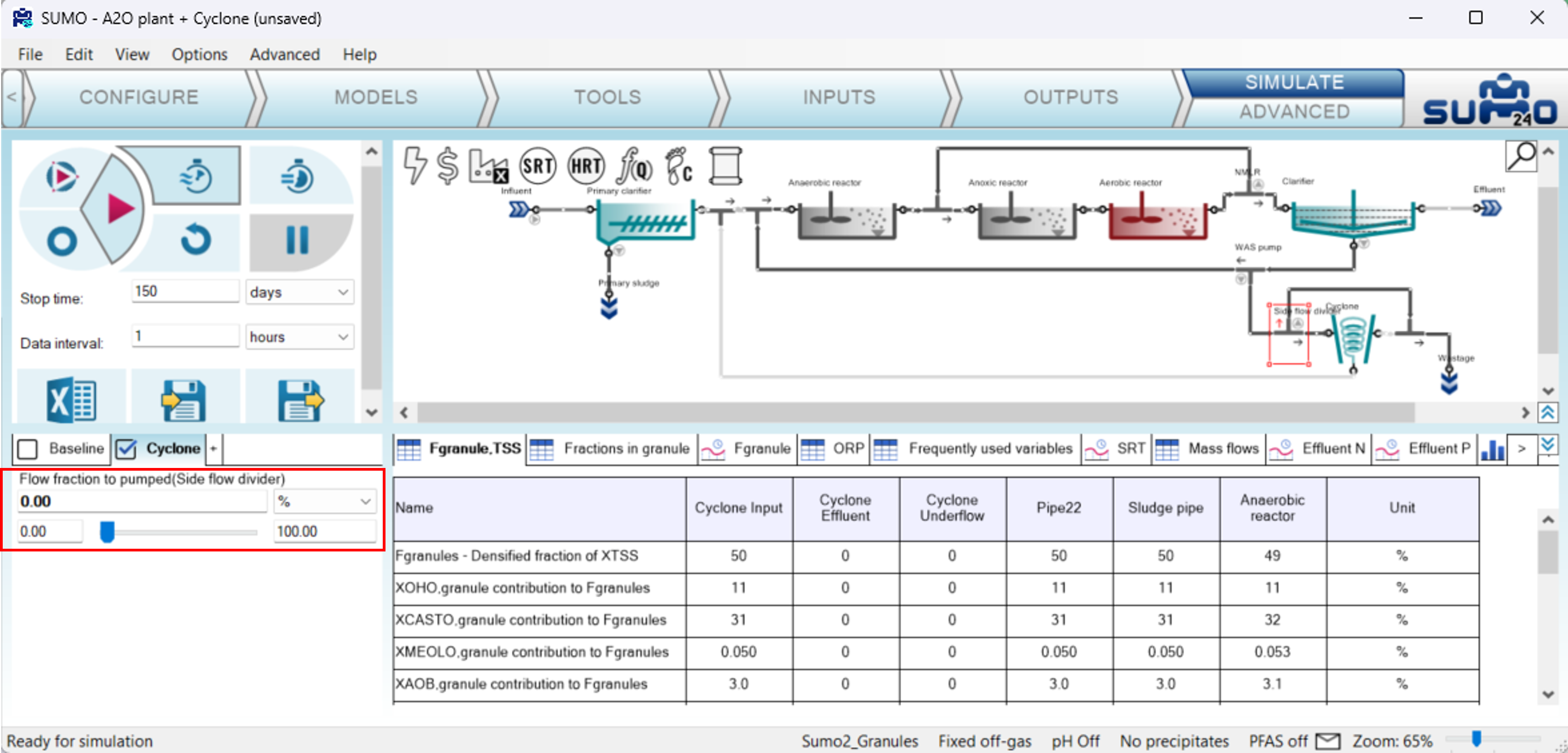
- Baseline scenario: flow fraction to pumped Side flow divider = 100%
- Cyclone scenario: flow fraction to pumped Side flow divider = 0%
¶ Calibrating influent characteristics
The model includes fractions to represent the amount of particulate inorganic (XINORG), particulate unbiodegradable (XU), particulate biodegradable (XB) and heterotrophs (XOHO) that are granular. The default values are 20%, 10%, 0% and 1%, respectively. The fractions are applied in the following manner: if the amount of influent XINORG is 75 mg/L then 15 mg/L (20%) will be assigned to XINORG,granule and the remaining 60 mg/L (80%) to regular “floccular” XINORG.
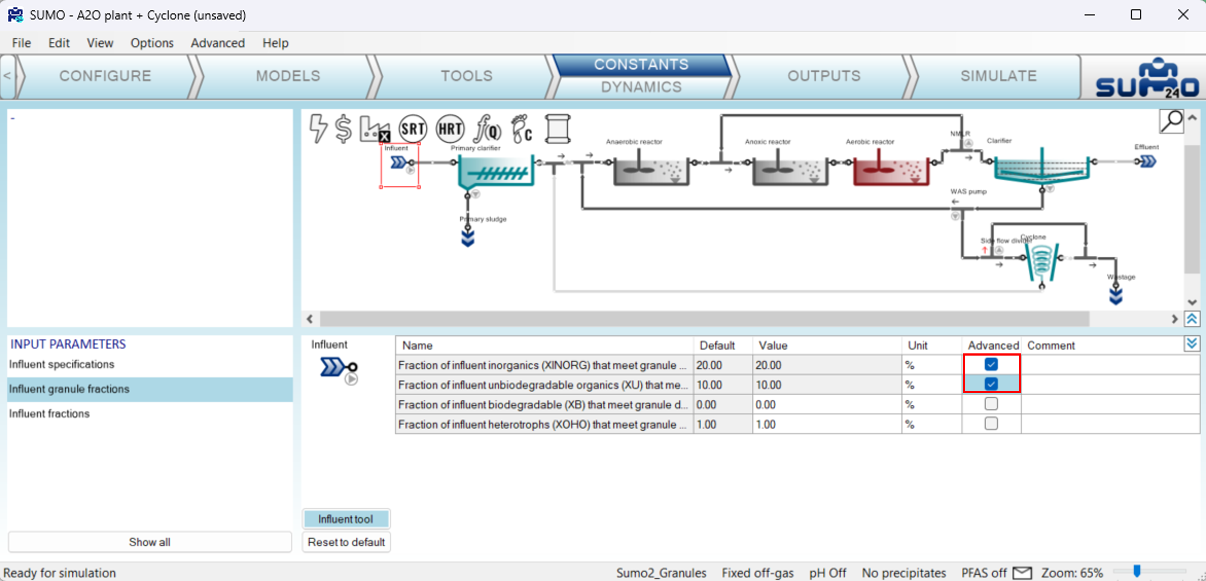
By including these in the scenarios we can use them to calibrate the amount unbiodegradable material that contributes to the densified fraction.
For example:
- Calculate the steady-state of the Baseline scenario with default parameters (note that with granular model it may take several minutes to reach steady-state) : the densified fraction is 6.1%
- Change the fraction of influent unbiodegradable organics (XU) that meets the granule definition from 10% to 5%
- Run a dynamic simulation for 100d : the Densified fraction is reduced to 5.1%.
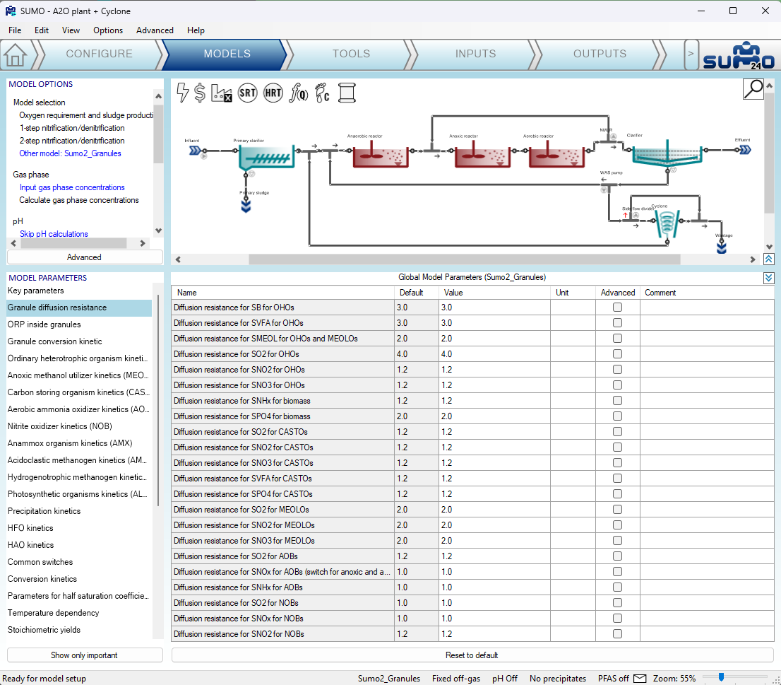
¶ Calibrating Diffusion Resistance (DR)
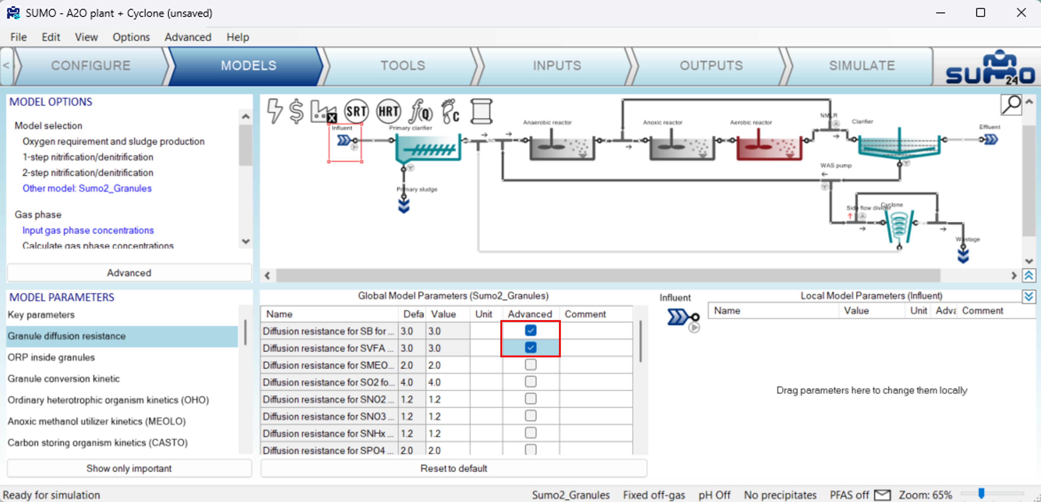
The diffusion resistance (DR) parameters are defined in the MODELS tab of the Sumo ribbon in the bottom left pane after selecting “Show all” under the heading “Granule diffusion resistance”. We can calibrate the impact of these parameters by selecting the “Scenario” boxes as shown below.
The following steps illustrate the sensitivity of the model results to the DR parameters:
- Calculate the steady-state of the Baseline scenario with default parameters (note that with granular model it may take several minutes to reach steady-state) : the densified fraction is 6.1%
- Change the DR for susbtrates SB and SVFA from 3 to 1.5
- Calculate the new steady-state: the Densified fraction is increased to 22.9%.
The same steps for the “Cyclone” scenario and including the changes to the diffusion resistance parameters from 3 to 1.5, we see the change in Densified fraction “Fgranules” increase from 55.8% to 68.1%.
¶ Oxidation-reduction potential (ORP)
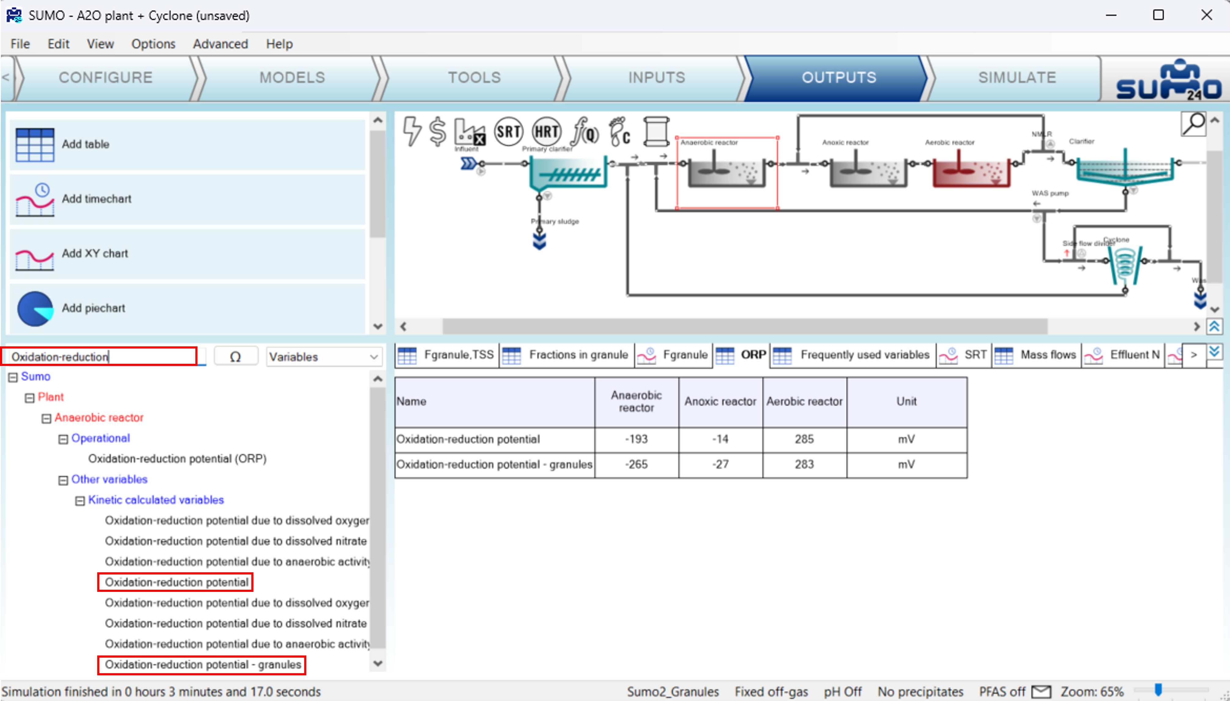
The model calculates a difference in ORP for fermentative organisms in the floc and the granules. The ORP for the flocs and granules can be viewed in a table by typing “Oxidation-reduction” into the dialog box in the bottom left pane of the OUTPUTS tab of the Sumo ribbon. As long as the “Variables” option is selected from the drop-down menu then the “Oxidation-reduction potential” for the flocs and granules should be displayed. As can be seen below, the ORP in the granules is lower than in the flocs.
¶ Cyclone operations calibration
The Cyclone operating parameters can be accessed in the INPUTS tab of the Sumo ribbon. The cyclone model is defined with only five parameters as previously described in Cyclone model specifics paragraph.
These parameters have to be calibrated based on the measurements around the cyclone and will impact the simulated Densified fraction.
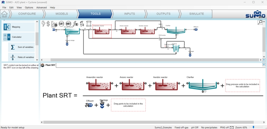
¶ Plant and granules SRT calculation
The plant SRT calculation can be calculated as usual in the TOOLS ribbon, selecting the “Sludge Retention Time” feature and selecting the proper units with drag and drop method.
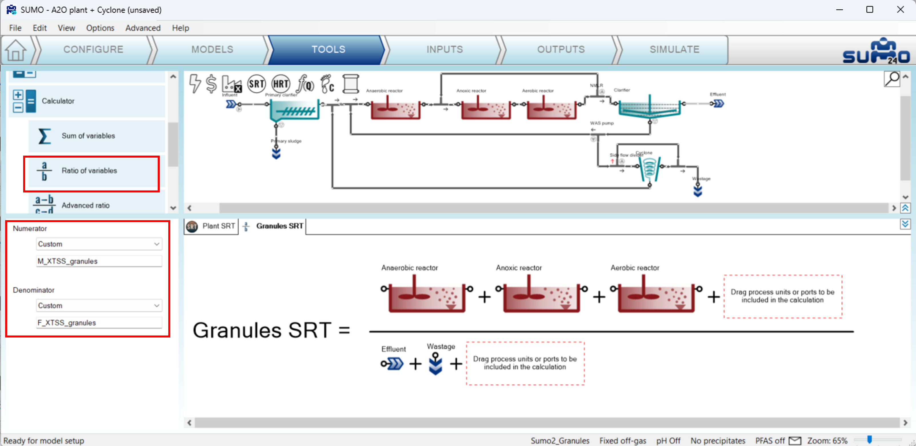
The calculation of granule SRT can be done on the basis of one of the granular TSS, as XTSS, granules. The “Ratio of variables” calculation has to be selected in the top left panel, and “custom” numerator and denominator variables should be set in the bottom left panel as “M_X_TSS_granules” and “F_X_TSS_granules” respectively. In the bottom right panel, the appropriate process units should be drag and drop at numerator and denominator.
In the following simulation with the cyclone activated, the process is intensified by increasing the WAS pumped flow from 300 m3/d to 900 m3/d. The SRT calculations results in 6.8d SRT for the plant and 15.5d SRT for granules.
